Lyapunov Analysis
Optimal control provides a powerful framework for formulating control problems using the language of optimization. But solving optimal control problems for nonlinear systems is hard! In many cases, we don't really care about finding the optimal controller, but would be satisfied with any controller that is guaranteed to accomplish the specified task. In many cases, we still formulate these problems using computational tools from optimization, and in this chapter we'll learn about tools that can provide guaranteed control solutions for systems that are beyond the complexity for which we can find the optimal feedback.
There are many excellent books on Lyapunov analysis; for instance
Lyapunov Functions
Let's start with our favorite simple example.
Stability of the Damped Pendulum

Recall that the equations of motion of the damped simple pendulum are given by \[ ml^2 \ddot{\theta} + mgl\sin\theta = -b\dot{\theta}, \] which I've written with the damping on the right-hand side to remind us that it is an external torque that we've modeled.
These equations represent a simple second-order differential equation; in chapter 2 we discussed at some length what was known about the solutions to this differential equation--in practice we do not have a closed-form solution for $\theta(t)$ as a function of the initial conditions. Since we couldn't provide a solution analytically, in chapter 2 we resorted to a graphical analysis, and confirmed the intuition that there are fixed points in the system (at $\theta = k\pi$ for every integer $k$) and that the fixed points at $\theta = 2\pi k$ are asymptotically stable with a large basin of attraction. The graphical analysis gave us this intuition, but can we actually prove this stability property? In a way that might also work for much more complicated systems?
One route forward was from looking at the total system energy (kinetic + potential), which we can write down: \[ E(\theta,\dot{\theta}) = \frac{1}{2} ml^2\dot{\theta}^2 - mgl \cos\theta. \] Recall that the contours of this energy function are the orbits of the undamped pendulum.

A natural route to proving the stability of the downward fixed points is by arguing that energy (almost always) decreases for the damped pendulum ($b>0$) and so the system will eventually come to rest at the minimum energy, $E = -mgl$, which happens at $\theta=2\pi k$. Let's make that argument slightly more precise.
Evaluating the time derivative of the energy reveals \[ \frac{d}{dt} E = \pd{E}{\theta}\dot\theta + \pd{E}{\dot\theta}\ddot\theta = \dot\theta(ml^2\ddot\theta + mgl\sin\theta) = - b\dot\theta^2 \le 0. \] So we know that energy will never increase, that energy is bounded, and that it obtains it's minima at the downward (stable) fixed points. Moreover, we now know that energy is strictly decreasing whenever $\dot\theta \neq 0$. We're getting close.
In order to show that the system converges asymptotically to some fixed point, we need one more observation. For non-fixed-point states with $\dot\theta = 0$, we have $\dot{E} = 0$, but only for an instant. A moment later, we'll have some non-zero velocity once again, and again start dissipating energy. All together, these arguments are sufficient to demonstrate that $\bx \rightarrow$ a fixed point as $t \rightarrow \infty$. We'll make this argument more general and more precise below.
This is an important example. It demonstrated that we could use a relatively simple function -- the total system energy -- to describe something about the long-term dynamics of the pendulum even though the actual trajectories of the system are (analytically) very complex. It also demonstrated one of the subtleties of using an energy-like function that is non-increasing (instead of strictly decreasing) to prove asymptotic stability.
Lyapunov functions generalize this notion of an energy function to more general systems, which might not be stable in the sense of some mechanical energy. If I can find any positive function, call it $V(\bx)$, that gets smaller over time as the system evolves, then I can potentially use $V$ to make a statement about the long-term behavior of the system. $V$ is called a Lyapunov function.
Recall that we defined three separate notions for stability of a fixed-point of a nonlinear system: stability i.s.L., asymptotic stability, and exponential stability. We can use Lyapunov functions to demonstrate each of these, in turn.
Lyapunov's Direct Method (for local stability)
Given a system $\dot{\bx} = f(\bx)$, with $f$ continuous, and for some region ${\cal D}$ around the origin (specifically an open subset of $\mathbf{R}^n$ containing the origin), if I can produce a scalar, continuously-differentiable function $V(\bx)$, such that \begin{gather*} V(\bx) > 0, \forall \bx \in {\cal D} \setminus \{0\} \quad V(0) = 0, \text{ and} \\ \dot{V}(\bx) = \pd{V}{\bx} f(\bx) \le 0, \forall \bx \in {\cal D} \setminus \{0\} \quad \dot{V}(0) = 0, \end{gather*} then the origin $(\bx = 0)$ is stable in the sense of Lyapunov (i.s.L.). [Note: the notation $A \setminus B$ represents the set $A$ with the elements of $B$ removed.]
If, additionally, we have $$\dot{V}(\bx) = \pd{V}{\bx} f(\bx) < 0, \forall \bx \in {\cal D} \setminus \{0\},$$ then the origin is (locally) asymptotically stable. And if we have $$\dot{V}(\bx) = \pd{V}{\bx} f(\bx) \le -\alpha V(x), \forall \bx \in {\cal D} \setminus \{0\},$$ for some $\alpha>0,$ then the origin is (locally) exponentially stable.
Note that for the sequel we will use the notation $V \succ 0$ to denote a positive-definite function, meaning that $V(0)=0$ and $V(\bx)>0,$ for all $\bx \ne 0$. We can use "positive definite in ${\cal D}$" if this applies $\forall x \in {\cal D}$. Similarly, we'll use $V \succeq 0$ for positive semi-definite, $V \prec 0$ for negative-definite functions, etc.
The intuition here is exactly the same as for the energy argument we made in the pendulum example: since $\dot{V}(x)$ is always zero or negative, the value of $V(x)$ will only get smaller (or stay the same) as time progresses. Inside the subset ${\cal D}$, for every $\epsilon$-ball, I can choose a $\delta$ such that $|x(0)|^2 < \delta \Rightarrow |x(t)|^2 < \epsilon, \forall t$ by choosing $\delta$ sufficiently small so that the sublevel set of $V(x)$ for the largest value that $V(x)$ takes in the $\delta$ ball is completely contained in the $\epsilon$ ball. Since the value of $V$ can only get smaller (or stay constant) in time, this gives stability i.s.L.. If $\dot{V}$ is strictly negative away from the origin, then it must eventually get to the origin (asymptotic stability). The exponential condition is implied by the fact that $\forall t>0, V(\bx(t)) \le V(\bx(0)) e^{-\alpha t}.$
Notice that the system analyzed above, $\dot{\bx}=f(\bx)$, did not have any control inputs. Lyapunov analysis is used to study either the passive dynamics of a system or the dynamics of a closed-loop system (e.g. the plant and controller connected in a feedback loop). We will see generalizations of the Lyapunov function ideas to input-output systems later in the text.
Global Stability
The notion of a fixed point being stable i.s.L. is inherently a local notion of stability (defined with $\epsilon$ and $\delta$ balls around the origin), but the notions of asymptotic and exponential stability can be applied globally. The Lyapunov theorems work for this case, too, with only minor modification.
Lyapunov analysis for global stability
Given a system $\dot{\bx} = f(\bx)$, with $f$ continuous, if I can produce a scalar, continuously-differentiable function $V(\bx)$, such that \begin{gather*} V(\bx) \succ 0, \\ \dot{V}(\bx) = \pd{V}{\bx} f(\bx) \prec 0, \text{ and} \\ V(\bx) \rightarrow \infty \text{ whenever } ||\bx||\rightarrow \infty,\end{gather*} then the origin $(\bx = 0)$ is globally asymptotically stable (G.A.S.).
If additionally we have that $$\dot{V}(\bx) \preceq -\alpha V(\bx),$$ for some $\alpha>0$, then the origin is globally exponentially stable.
The new condition, on the behavior as $||\bx|| \rightarrow \infty$ is known as "radially unbounded", and is required to make sure that trajectories cannot diverge to infinity even as $V$ decreases; it is only required for global stability analysis. This radially unbounded condition is sufficient but is not necessary; other conditions can potentially be invoked to guarantee that the system avoids this pathology. More essential is that the resulting trajectory $\bx(t)$ is bounded for all $t$.
LaSalle's Invariance Principle
Perhaps you noticed the disconnect between the statement above and the argument that we made for the stability of the pendulum. In the pendulum example, using the mechanical energy resulted in a Lyapunov function time derivative that was only negative semi-definite, but we eventually argued that the fixed points were asymptotically stable. That took a little extra work, involving an argument about the fact that the fixed points were the only place that the system could stay with $\dot{E}=0$; every other state with $\dot{E}=0$ was only transient. We can formalize this idea for the more general Lyapunov function statements--it is known as LaSalle's Theorem.
LaSalle's Theorem
Given a system $\dot{\bx} = f(\bx)$ with $f$ continuous. If we can produce a scalar function $V(\bx)$ with continuous derivatives for which we have $$V(\bx) \succ 0,\quad \dot{V}(\bx) \preceq 0,$$ and $V(\bx)\rightarrow \infty$ as $||\bx||\rightarrow \infty$, then $\bx$ will converge to the largest invariant set where $\dot{V}(\bx) = 0$.
To be clear, an invariant set, ${\cal G}$, of the dynamical
system is a set for which $\bx(0)\in{\cal G} \Rightarrow \forall t>0,
\bx(t) \in {\cal G}$. In other words, once you enter the set you never
leave. The "largest invariant set" with $\dot{V}(\bx) = 0$ need not be
connected; in fact for the pendulum example each fixed point is an
invariant set with $\dot{V} = 0$, so the largest invariant set is the
union of all the fixed points of the system. There are also variants of
LaSalle's Theorem which work over a region. For example, the total energy of the
pendulum does not actually satisfy the radially-unbounded condition (the energy is
finite as $\theta \rightarrow \infty$), but observing that $\bx(t)$ is bounded for
all initial conditions is sufficient to invoke a variant of LaSalle's theorem
Finding a Lyapunov function which $\dot{V} \prec 0$ is more difficult than finding one that has $\dot{V} \preceq 0$. LaSalle's theorem gives us the ability to make a statement about asymptotic stability even in this case. In the pendulum example, every state with $\dot\theta=0$ had $\dot{E}=0$, but only the fixed points are in the largest invariant set.
Swing-up for the Cart-Pole System
Recall the example of using partial-feedback linearization to generate a swing-up controller for the cart-pole system. We first examined the dynamics of the pole (pendulum) only, by writing it's energy: $$E(\bx) = \frac{1}{2}\dot\theta^2 - \cos\theta,$$ desired energy, $E^d = 1$, and the difference $\tilde{E}(\bx) = E(\bx) - E^d.$ We were able to show that our proposed controller produced $$\dot{\tilde{E}} = -k \dot\theta^2 \cos^2\theta \tilde{E},$$ where $k$ is a positive gain that we get to choose. And we said that was good!
Now we have the tools to understand that really we have a Lyapunov function $$V(\bx) = \frac{1}{2}\tilde{E}^2(\bx),$$ and what we have shown is that $\dot{V} \le 0$. By LaSalle, we can only argue that the closed-loop system will converge to the largest invariant set, which here is the entire homoclinic orbit: $\tilde{E}(\bx) = 0$. We have to switch to the LQR controller in order to stabilize the upright.
As you can see from the plots, $\dot{V}(\bx)$ ends up being a quite non-trivial function! We'll develop the computational tools for verifying the Lyapunov/LaSalle conditions for systems of this complexity in the upcoming sections.
Relationship to the Hamilton-Jacobi-Bellman equations
At this point, you might be wondering if there is any relationship between Lyapunov functions and the cost-to-go functions that we discussed in the context of dynamic programming. After all, the cost-to-go functions also captured a great deal about the long-term dynamics of the system in a scalar function. We can see the connection if we re-examine the HJB equation \[ 0 = \min_\bu \left[ \ell(\bx,\bu) + \pd{J^*}{\bx}f(\bx,\bu). \right] \]Let's imagine that we can solve for the optimizing $\bu^*(\bx)$, then we are left with $ 0 = \ell(\bx,\bu^*) + \pd{J^*}{\bx}f(\bx,\bu^*) $ or simply \[ \dot{J}^*(\bx) = -\ell(\bx,\bu^*) \qquad \text{vs} \qquad \dot{V}(\bx) \preceq 0. \] In other words, in optimal control we must find a cost-to-go function which matches this gradient for every $\bx$; that's very difficult and involves solving a potentially high-dimensional partial differential equation. By contrast, Lyapunov analysis is asking for much less - any function which is going downhill (at any rate) for all states. This can be much easier, for theoretical work, but also for our numerical algorithms. Also note that if we do manage to find the optimal cost-to-go, $J^*(\bx)$, then it can also serve as a Lyapunov function so long as $\ell(\bx,\bu^*(\bx)) \succeq 0$.
Lyapunov functions for estimating regions of attraction
There is another very important connection between Lyapunov functions and the concept of an invariant set: any sublevel set of a Lyapunov function is also an invariant set. This gives us the ability to use sublevel sets of a Lyapunov function as approximations of the region of attraction for nonlinear systems. For a locally attractive fixed point, $\bx^*$, the region of attraction to $\bx^*$ is the largest set ${\cal D} \subseteq {\cal X}$ for which $\bx(0) \in {\cal D} \Rightarrow \lim_{t\rightarrow \infty} \bx(t) = \bx^*.$ Regions of attraction are always open, connected, and invariant sets (with boundaries ).
Lyapunov invariant set and region of attraction theorem
Given a system $\dot{\bx} = f(\bx)$ with $f$ continuous, if we can find a scalar function $V(\bx) \succ 0$ and a bounded sublevel set $${\cal G}: \{ \bx | V(\bx) \le \rho \}$$ on which $$\forall \bx \in {\cal G}, \dot{V}(\bx) \preceq 0,$$ then ${\cal G}$ is an invariant set. By LaSalle, $\bx$ will converge to the largest invariant subset of ${\cal G}$ on which $\dot{V}=0$.
If $\dot{V}(\bx) \prec 0$ in ${\cal G}$, then the origin is locally asymptotically stable and furthermore the set ${\cal G}$ is inside the region of attraction of this fixed point. Alternatively, if $\dot{V}(\bx) \preceq 0$ in ${\cal G}$ and $\bx = 0$ is the only invariant subset of ${\cal G}$ where $\dot{V}=0$, then the origin is asymptotically stable and the set ${\cal G}$ is inside the region of attraction of this fixed point.
Region of attraction for a one-dimensional system
Consider the first-order, one-dimensional system $\dot{x} = -x + x^3.$ We can quickly understand this system using our tools for graphical analysis.

In the vicinity of the origin, $\dot{x}$ looks like $-x$, and as we move away it looks increasingly like $x^3$. There is a stable fixed point at the origin and unstable fixed points at $\pm 1$. In fact, we can deduce visually that the region of attraction to the stable fixed point at the origin is $\bx \in (-1,1)$. Let's see if we can demonstrate this with a Lyapunov argument.
First, let us linearize the dynamics about the origin and use the Lyapunov equation for linear systems to find a candidate $V(\bx)$. Since the linearization is $\dot{x} = -x$, if we take ${\bf Q}=1$, then we find ${\bf P}=\frac{1}{2}$ is the positive definite solution to the algebraic Lyapunov equation (\ref{eq:algebraic_lyapunov}). Proceeding with $$V(\bx) = \frac{1}{2} x^2,$$ we have $$\dot{V} = x (-x + x^3) = -x^2 + x^4.$$ This function is zero at the origin, negative for $|x| < 1$, and positive for $|x| > 1$. Therefore we can conclude that the sublevel set $V < \frac{1}{2}$ is invariant and the set $x \in (-1,1)$ is inside the region of attraction of the nonlinear system. In fact, this estimate is tight.
Robustness analysis using "common Lyapunov functions"
While we will defer most discussions on robustness analysis until later in the notes, the idea of a common Lyapunov function, which we introduced briefly for linear systems in the example above, can be readily extended to nonlinear systems and region of attraction analysis. Imagine that you have a model of a dynamical system but that you are uncertain about some of the parameters. For example, you have a model of a quadrotor, and are fairly confident about the mass and lengths (both of which are easy to measure), but are not confident about the moment of inertia. One approach to robustness analysis is to define a bounded uncertainty, which could take the form of $$\dot{\bx} = f_\alpha(\bx), \quad \alpha_{min} \le \alpha \le \alpha_{max},$$ with $\alpha$ a vector of uncertain parameters in your model. Richer specifications of the uncertainty bounds are also possible, but this will serve for our examples.
In standard Lyapunov analysis, we are searching for a function that goes downhill for all $\bx$ to make statements about the long-term dynamics of the system. In common Lyapunov analysis, we can make many similar statements about the long-term dynamics of an uncertain system if we can find a single Lyapunov function that goes downhill for all possible values of $\alpha$. If we can find such a function, then we can use it to make statements with all of the variations we've discussed (local, regional, or global; in the sense of Lyapunov, asymptotic, or exponential).
A one-dimensional system with gain uncertainty
Let's consider the same one-dimensional example used above, but add an uncertain parameter into the dynamics. In particular, consider the system: $$\dot{x} = -x + \alpha x^3, \quad \frac{3}{4} < \alpha < \frac{3}{2}.$$ Plotting the graph of the one-dimensional dynamics for a few values of $\alpha$, we can see that the fixed point at the origin is still stable, but the robust region of attraction to this fixed point (shaded in blue below) is smaller than the region of attraction for the system with $\alpha=1$.

Taking the same Lyapunov candidate as above, $V = \frac{1}{2} x^2$, we have $$\dot{V} = -x^2 + \alpha x^4.$$ This function is zero at the origin, and negative for all $\alpha$ whenever $x^2 > \alpha x^4$, or $$|x| < \frac{1}{\sqrt{\alpha_{max}}} = \sqrt{\frac{2}{3}}.$$ Therefore, we can conclude that $|x| < \sqrt{\frac{2}{3}}$ is inside the robust region of attraction of the uncertain system.
Not all forms of uncertainty are as simple to deal with as the gain uncertainty in that example. For many forms of uncertainty, we might not even know the location of the fixed points of the uncertain system. In this case, we can often still use common Lyapunov functions to give some guarantees about the system, such as guarantees of robust set invariance. For instance, if you have uncertain parameters on a quadrotor model, you might be ok with the quadrotor stabilizing to a pitch of $0.01$ radians, but you would like to guarantee that it definitely does not flip over and crash into the ground.
A one-dimensional system with additive uncertainty
Now consider the system: $$\dot{x} = -x + x^3 + \alpha, \quad -\frac{1}{4} < \alpha < \frac{1}{4}.$$ Plotting the graph of the one-dimensional dynamics for a few values of $\alpha$, this time we can see that the fixed point is not necessarily at the origin; the location of the fixed point moves depending on the value of $\alpha$. But we should be able to guarantee that the uncertain system will stay near the origin if it starts near the origin, using an invariant set argument.

Taking the same Lyapunov candidate as above, $V = \frac{1}{2} x^2$, we have $$\dot{V} = -x^2 + x^4 + \alpha x.$$ This Lyapunov function allows us to easily verify, for instance, that $V \le \frac{1}{3}$ is a robust invariant set, because whenever $V = \frac{1}{3}$, we have $$\forall \alpha \in [\alpha_{min},\alpha_{max}],\quad \dot{V}(x,\alpha) < 0.$$ Therefore $V$ can never start at less than one-third and cross over to greater than one-third. To see this, see that $$ V=\frac{1}{3} \quad \Rightarrow \quad x = \pm \sqrt{\frac{2}{3}} \quad \Rightarrow \quad \dot{V} = -\frac{2}{9} \pm \alpha \sqrt{\frac{2}{3}} < 0, \forall \alpha \in \left[-\frac{1}{4},\frac{1}{4} \right]. $$ Note that not all sublevel sets of this invariant set are invariant. For instance $V < \frac{1}{32}$ does not satisfy this condition, and by visual inspection we can see that it is in fact not robustly invariant.
Barrier functions
Lyapunov functions are used to certify stability or to establish invariance of a region. But the same conditions can be used to certify that the state of a dynamical system will not visit some region of state space. This can be useful for e.g. verifying that your autonomous car will not crash or, perhaps, that your walking robot will not fall down. When used this way, we call the associated functions, $\mathcal{B}(\bx)$, "barrier functions".
Barrier functions
Given a continuously-differentiable dynamical system described by $\dot{\bx} = {\bf f}(\bx)$, if I can find a function $\mathcal{B}(\bx)$ such that $\forall \bx, \dot{\mathcal{B}}(\bx) \le 0$, then the system will never visit states with $\mathcal{B}(\bx(t)) > \mathcal{B}(\bx(0)).$
In particular, if we ensure that $\forall \bx$ in "failure" regions of state space, we have $\mathcal{B}(\bx) > 0$, then the level-set $\mathcal{B}(\bx) = 0$ can serve as a barrier certifying that trajectories starting with initial conditions with $\mathcal{B}(\bx) < 0$ will never enter the failure set.
Natural extensions exist for certifying these conditions over a region, considering piecewise-polynomial dynamics, worse-case robustness, etc.
Lyapunov analysis with convex optimization
One of the primary limitations in Lyapunov analysis as I have presented it so far is that it is potentially very difficult to come up with suitable Lyapunov function candidates for interesting systems, especially for underactuated systems. ("Underactuated" is almost synonymous with "interesting" in my vocabulary.) Even if somebody were to give me a Lyapunov candidate for a general nonlinear system, the Lyapunov conditions can be difficult to check -- for instance, how would I check that $\dot{V}$ is strictly negative for all $\bx$ except the origin if $\dot{V}$ is some arbitrarily complicated nonlinear function over a vector $\bx$?
In this section, we'll look at some computational approaches to verifying the Lyapunov conditions, and even to searching for (the coefficients of) the Lyapunov functions themselves.
If you're imagining numerical algorithms to check the Lyapunov conditions
for complicated Lyapunov functions and complicated dynamics, the first
thought is probably that we can evaluate $V$ and $\dot{V}$ at a large number
of sample points and check whether $V$ is positive and $\dot{V}$ is
negative. This
does work, and could potentially be combined with some smoothness or
regularity assumptions to generalize beyond the sample points.
Linear systems
The Lyapunov conditions we've explored above take a particularly nice form for linear systems.
Lyapunov analysis for stable linear systems
Imagine you have a linear system, $\dot\bx = {\bf A}\bx$, and can find a Lyapunov function $$V(\bx) = \bx^T {\bf P} \bx, \quad {\bf P} = {\bf P^T} \succ 0,$$ which also satisfies $$\dot{V}(\bx) = \bx^T {\bf PA} \bx + \bx^T {\bf A}^T {\bf P}\bx \prec 0.$$ Then the origin is globally exponentially stable.
Note that the radially-unbounded condition is satisfied by ${\bf P} \succ 0$, and that the derivative condition is equivalent to the matrix condition $${\bf PA} + {\bf A}^T {\bf P} \prec 0.$$
For stable linear systems the existence of a quadratic Lyapunov function is actually a necessary (as well as sufficient) condition. Furthermore, if $\bA$ is stable, then a Lyapunov function can always be found by finding the positive-definite solution to the matrix Lyapunov equation \begin{equation}{\bf PA} + {\bf A}^T{\bf P} = - {\bf Q},\label{eq:algebraic_lyapunov} \end{equation} for any ${\bf Q}={\bf Q}^T\succ 0$.
This is a very powerful result - for nonlinear systems it will be potentially difficult to find a Lyapunov function, but for linear systems it is straightforward. In fact, this result is often used to propose candidate Lyapunov functions for nonlinear systems, e.g., by linearizing the equations and solving a local linear Lyapunov function which should be valid in the vicinity of a fixed point.
Lyapunov analysis for linear systems has an extremely important connection to convex optimization. In particular, we could have also formulated the Lyapunov conditions for linear systems above using semi-definite programming (SDP). Semidefinite programming is a subset of convex optimization -- an extremely important class of problems for which we can produce efficient algorithms that are guaranteed find the global optima solution (up to a numerical tolerance and barring any numerical difficulties).
If you don't know much about convex optimization or want a quick refresher, please take a few minutes to read the optimization preliminaries in the appendix. The main requirement for this section is to appreciate that it is possible to formulate efficient optimization problems where the constraints include specifying that one or more matrices are positive semi-definite (PSD). These matrices must be formed from a linear combination of the decision variables. For a trivial example, the optimization $$\min_a a,\quad \subjto \begin{bmatrix} a & 0 \\ 0 & 1 \end{bmatrix} \succeq 0,$$ returns $a = 0$ (up to numerical tolerances).
The value in this is immediate for linear systems. For example, we can formulate the search for a Lyapunov function for the linear system $\dot\bx = {\bf A} \bx$ by using the parameters ${\bf p}$ to populate a symmetric matrix ${\bf P}$ and then write the SDP: \begin{equation} \find_{\bf p} \quad \subjto \quad {\bf P} \succeq 0, \quad {\bf PA} + {\bf A}^T {\bf P} \preceq 0.\label{eq:lyap} \end{equation} Note that you would probably never use that particular formulation, since there specialized algorithms for solving the simple Lyapunov equation which are more efficient and more numerically stable. But the SDP formulation does provide something new -- it will give us our first example of robustness analysis. In particular, we can now easily formulate the search for a "common Lyapunov function" for uncertain linear systems.
Common Lyapunov analysis for linear systems
Suppose you have a system governed by the equations $\dot\bx = {\bf A}\bx$, where the matrix ${\bf A}$ is unknown, but its uncertain elements can be bounded. There are a number of ways to write down this uncertainty set; let us choose to write this by describing ${\bf A}$ as the convex combination of a number of known matrices, $${\bf A} = \sum_{i} \beta_i {\bf A}_i, \quad \sum_i \beta_i = 1, \quad \forall i, \beta_i > 0.$$ This is just one way to specify the uncertainty; geometrically it is describing a polygon of uncertain parameters (in the space of elements of ${\bf A}$ with each ${\bf A}_i$ as one of the vertices in the polygon.

Now we can formulate the search for a common Lyapunov function using \[ \find_{\bf p} \quad \subjto \quad {\bf P} \succeq 0, \quad \forall_i, {\bf PA}_i + {\bf A}_i^T {\bf P} \preceq 0.\] The solver will then return a matrix ${\bf P}$ which satisfies all of the constraints, or return saying "problem is infeasible". It can easily be verified that if ${\bf P}$ satisfies the Lyapunov condition at all of the vertices, then it satisfies the condition for every ${\bf A}$ in the set: \[ {\bf P}(\sum_i \beta_i {\bf A}_i) + (\sum_i \beta_i {\bf A}_i)^T {\bf P} = \sum_i \beta_i ({\bf P A}_i + {\bf A}_i^T {\bf P}) \preceq 0, \] since $\forall i$, $\beta_i > 0$. Note that, unlike the simple Lyapunov equation for a known linear system, this condition being satisfied is a sufficient but not a necessary condition -- it is possible that the set of uncertain matrices ${\bf A}$ is robustly stable, but that this stability cannot be demonstrated with a common quadratic Lyapunov function.
You can try this example for yourself in
As always, make sure that you open up the code and take a look.
Note that the argument above does not actually make use of the $\sum_i \beta_i = 1;$ that assumption can be safely removed. So really, our common Lyapunov function, when found, has certified the convex cone with the $A_i$ matrices as the extreme rays. This is not surprising, since if we have any linear system/Lyapunov quadratic form pair $A, P$, then $P$ also confirms that $\beta A$ is stable for any $\beta > 0.$ Multiplying a system matrix by a scalar will not change the sign of its eigenvalues.
There are many small variants of this result that are potentially of
interest. For instance, a very similar set of conditions can certify
"mean-square stability" for linear systems with multiplicative noise
(see e.g.
This example is very important because it establishes a connection between Lyapunov functions and (convex) optimization. But so far we've only demonstrated this connection for linear systems where the PSD matrices provide a magical recipe for establishing the positivity of the (quadratic) functions for all $\bx$. Is there any hope of extending this type of analysis to more general nonlinear systems? Surprisingly, it turns out that there is.
Global analysis for polynomial systems
Sums of squares (SOS) optimization provides a natural generalization of the SDP formulation to nonlinear systems. In SDP, we were allowed to write constraints of the form, ${\bf P} \succeq 0$. In sums of squares optimization, we generalize this to writing constraints of the form "$p_\balpha(\bx)$ is SOS", where $p(\bx)$ is a polynomial with coefficients $\balpha$. Let's examine this in the specific context of Lyapunov functions.
In linear systems, we searched over $V(\bx) = \bx^T {\bf P} \bx, {\bf P} \succeq 0.$ In the nonlinear generalization, we search over $$V(\bx) = {\bf m}^T(\bx) {\bf P} {\bf m}(\bx),\quad {\bf P} \succeq 0,$$ with ${\bf m}(\bx)$ a set of nonlinear basis functions. This is a linear (in the parameters ${\bf P}$) function approximator which is guaranteed to be strictly positive by virtue of being a sum of squares. While the positivity of this sums of squares is valid for any choice of ${\bf m}(\bx)$, the recipe is particularly powerful for polynomials, because for any polynomial, $p(\bx)$, we can confirm its positivity by creating a surrogate sums-of-squares representation, where we have strong recipes for automatically choosing good bases ${\bf m}(\bx)$ given a polynomial $p(\bx)$, and we can constrain that $p(\bx) = {\bf m}^T(\bx) {\bf P} {\bf m}(\bx)$ with linear constraints relating the coefficients of $p(\bx)$ with the coefficient in ${\bf P}$.
This suggests that it may be possible to generalize the optimization approach using SDP to search for Lyapunov functions for linear systems to searching for Lyapunov functions for nonlinear systems: $\dot\bx = \bf{f}(\bx),$ where $\bf{f}$ is a vector-valued polynomial function. Importantly, if $V(\bx)$ is polynomial, and $\bf{f}(\bx)$ is polynomial, then $\dot{V}(\bx) = \pd{V}{\bx}{\bf f}(\bx)$ is also polynomial.
If we parameterize a fixed-degree Lyapunov candidate as a polynomial with unknown coefficients, e.g., \[ V_\alpha(\bx) = \alpha_0 + \alpha_1 x_1 + \alpha_2 x_2 + \alpha_3 x_1x_2 + \alpha_4 x_1^2 + ..., \] then we can formulate the optimization: \begin{align*} \find_\alpha, \quad \subjto \quad& V_\alpha(\bx) \sos, \quad V_\alpha(0) = 0 \\ & -\dot{V}_\alpha(\bx) = -\pd{V_\alpha}{\bx} f(\bx) \sos. \end{align*} Because this is a convex optimization, the solver will return a solution if one exists, and this solution would certify stability i.s.L. of the origin. Note that I don't actually need to include the constraint $\dot{V}_\alpha({\bf 0}) = 0$; if $V_\alpha$ is a smooth function, is zero at zero, and is positive for all $\bx$, then this already implies that $\pd{V_\alpha}{\bx} = 0.$
If we wish to demonstrate (global) asymptotic stability, then we can write the constraint $\dot{V}_\alpha(\bx) \prec 0$ as $$-\dot{V}_\alpha(\bx) - \epsilon \bx^T\bx \text{ is SOS,}$$ where $\epsilon$ is a small positive constant that need only be larger than the numerical tolerances of the solver. The conditions for exponential stability fit easily, too.
Verifying a Lyapunov candidate via SOS
This example is example 7.2 from
The numerical solution can be written in a few lines of code, and is a convex optimization.
Searching for a Lyapunov function via SOS
Verifying a candidate Lyapunov function is all well and good, but the real excitement starts when we use optimization to find the Lyapunov function. In the following code, we parameterize $V(x)$ as the polynomial containing all monomials up to degree 2, with the coefficients as decision variables: $$V(x) = c_0 + c_1x_0 + c_2x_1 + c_3x_0^2 + c_4 x_0x_1 + c_5 x_1^2.$$ We will set the scaling (arbitrarily) to avoid numerical issues by setting $V(0)=0$, $V([1,0]) = 1$. Then we write: \begin{align*} \find_{\bc} \ \ \subjto \ \ & V\text{ is sos, } \\ & -\dot{V} \text{ is sos.}\end{align*}
Up to numerical convergence tolerance, it discovers the same coefficients that we chose above (zeroing out the unnecessary terms).
Cart-pole swingup (again)
In the cart-pole swingup example, we took $$V(\bx) = \frac{1}{2} \tilde{E}^2(\bx) = \frac{1}{2} (\frac{1}{2}\dot\theta^2 - \cos\theta - 1)^2.$$ This is clearly a sum of squares. Furthermore, we showed that $$\dot{V}(\bx) = - \dot\theta^2 \cos^2\theta \tilde{E}^2(\bx),$$ which is also a sum of squares. So the proposal of using sums-of-squares optimization is not so different, actually, than the recipes that nonlinear control theorists have been using (on pen and paper) for years.
The SOS approach, as presented so far, could take only the nonlinear basis, ${\bf m}(\bx)$ for the candidate Lyapunov function, the degree of that Lyapunov function, and the closed-loop nonlinear dynamics; it would recover the parameters of a Lyapunov function and a certificate demonstrating the $V(\bx)$ and $-\dot{V}(\bx)$ are SOS. In this case, I would need a basis vector that includes many more monomials: $[1, \dot\theta, \cos\theta, ..., \dot\theta^3, ... ]^T.$
You might have noticed that I did something sneaky in here. The dynamics of the cart-pole are not simply polynomial in $\bx$; there are trigonometric terms in there. Setting up the equality constraints in an optimization requires more complicated term matching when trigonometric functions are involved, but the recipe still works. We will discuss this in more detail below.
It is important to remember that there are a handful of gaps which
make the existence of this solution a sufficient condition (to guarantee
that $V(\bx)$ is a Lyapunov function for $\bf{f}(\bx)$) instead of a necessary
one. First, there is no guarantee that a stable polynomial system can be
verified using a polynomial Lyapunov function (of any degree), and in fact
there are known counter-examples
Despite these caveats, I have found this formulation to be surprisingly effective in practice. Intuitively, I think that this is because there is relatively a lot of flexibility in the Lyapunov conditions -- if you can find one function which is a Lyapunov function for the system, then there are also many "nearby" functions which will satisfy the same constraints. This is the fundamental benefit of changing the equality in the HJB into an inequality in Lyapunov analysis.
Region of attraction estimation for polynomial systems
Now we have arrived at the tool that I believe can be a work-horse for many serious robotics applications. Most of our robots are not actually globally stable. That's not because they are robots -- if you push me hard enough, I will fall down, too! Asking for global stability is too much, but we can instead certify that our closed-loop systems behave well over a sufficiently large region of state space (and potentially for a range of possible parameters or disturbances). One of the simplest versions of this is estimating the region of attraction to a fixed point.
Sums-of-squares optimization effectively gives us an oracle which we can ask: is this polynomial positive for all $\bx$? To use this for regional analysis, we have to figure out how to modify our questions to the oracle so that the oracle will say "yes" or "no" when we ask if a function is positive over a certain region which is a subset of $\Re^n$. That trick is called the S-procedure. It is closely related to the Lagrange multipliers from constrained optimization, and has deep connections to "Positivstellensatz" from algebraic geometry.
The S-procedure
Consider a scalar polynomial, $p(\bx)$, and a semi-algebraic set $g(\bx) \le 0$. The term "semi-algebraic set" just means the set is defined by polynomial inequalities (here $g(\bx) \le 0$). If I can find a polynomial "multiplier", $\lambda(\bx)$, such that \[ p(\bx) + \lambda^T(\bx) g(\bx) \sos, \quad \text{and} \quad \lambda(\bx) \sos, \] then this is sufficient to demonstrate that $$p(\bx)\ge 0 \quad \forall \bx \in \{ \bx~|~g(\bx) \le 0 \}.$$ To convince yourself, observe that when $g(\bx) \le 0$, it is only harder to be positive, but when $g(\bx) > 0$, it is possible for the combined function to be SOS even if $p(\bx)$ is negative. We will sometimes find it convenient to use the short-hand: $$g(\bx) \le 0 \Rightarrow p(\bx) \ge 0$$ to denote the implication certified by the S-procedure, e.g. whenever $g(\bx) \le 0$, we have $p(\bx) \ge 0.$
We can also handle equality constraints with only a minor modification -- we no longer require the multiplier to be positive. If I can find a polynomial "multiplier", $\lambda(\bx)$, such that \[p(\bx) + \lambda^T(\bx) g(\bx) \sos \] then this is sufficient to demonstrate that $$p(\bx)\ge 0 \quad \forall \bx \in \{ \bx | g(\bx) = 0 \}.$$ Note the difference: for $g(\bx)\le 0$ we needed $\lambda(\bx) \ge 0$, but for $g(\bx) = 0$, $\lambda(\bx)$ can be arbitrary. The intuition is that $\lambda(\bx)$ can add arbitrary positive terms to help me be SOS, but those terms contribute nothing precisely when $g(\bx)=0$.
Basic region of attraction formulation
The S-procedure gives us the tool we need to evaluate positivity only over a region of state space, which is precisely what we need to certify the Lyapunov conditions for a region-of-attraction analysis. Let us start with a positive-definite polynomial Lyapunov candidate, $V(\bx) \succ 0$, then we can write the Lyapunov conditions: $$\dot{V}(\bx) \prec 0 \quad \forall \bx \in \{ \bx | V(\bx) \le \rho \},$$ using sums-of-squares and the S-procedure: $$-\dot{V}(\bx) + \lambda(\bx)(V(\bx) - \rho) \text{ is SOS,} \quad \text{and} \quad \lambda(\bx) \text{ is SOS},$$ where $\lambda(\bx)$ is a multiplier polynomial with free coefficients that are to be solved for in the optimization. Note that we've carefully chosen to denote the region of interest using a sub-level set of $V(\bx)$, so that we can be sure that region is also an invariant set (one of the requirements for the region of attraction analysis described above).
I think it's easiest to see the details in an example.
Region of attraction for the one-dimensional cubic system
Let's return to our example from above: \[ \dot{x} = -x + x^3 \] and try to use SOS optimization to demonstrate that the region of attraction of the fixed point at the origin is $x \in (-1,1)$, using the Lyapunov candidate $V(x) = x^2.$
First, define the multiplier polynomial, \[ \lambda(x) = c_0 + c_1 x + c_2 x^2. \] Then define the optimization \begin{align*} \find_{\bf c} \quad & \\ \subjto \quad& - \dot{V}(x) + \lambda(x) (V(x)-1) \sos \\ & \lambda(x) \sos \end{align*}
You can try these examples for yourself in
In this example, we only verified that the one-sublevel set of the pre-specified Lyapunov candidate is negative (certifying the ROA that we already understood). More generally, we can replace the 1-sublevel set with any constant value $\rho$. It is tempting to try to make $\rho$ a decision variable that we could optimize, but this would make the optimization problem non-convex because we would have terms like $\rho c_0$, $\rho c_1 x$, which are bilinear in the decision variables. We need the sums-of-squares constraints to be only linear in the decision variables.
Fortunately, because the problem is convex with $\rho$ fixed (and therefore can be solved reliably), and $\rho$ is just a scalar, we can perform a simple line search on $\rho$ to find the largest value for which the convex optimization returns a feasible solution. This will be our estimate for the region of attraction.
There are a number of variations to this basic formulation; I will describe a few of them below. There are also important ideas like rescaling and degree-matching that can have a dramatic effect on the numerics of the problem, and potentially make them much better for the solvers. But you do not need to master them all in order to use the tools effectively.
The equality-constrained formulation
Here is one important variation for finding the level set of a
candidate region of attraction, which turns an inequality in the
S-procedure into an equality. This formulation is jointly
convex in $\lambda(\bx)$ and $\rho$, so one can optimize them in a
single convex optimization. It appeared informally in an example in
Under the assumption that the Hessian of $\dot{V}(\bx)$ is negative-definite at the origin (which is easily checked), we can write \begin{align*} \max_{\rho, \lambda(\bx)} & \quad \rho \\ \subjto & \quad (\bx^T\bx)^d (V(\bx) - \rho) + \lambda^T(\bx) \dot{V}(\bx) \text{ is SOS},\end{align*} with $d$ a fixed positive integer. As you can see, $\rho$ no longer multiplies the coefficient of $\lambda(\bx)$. But why does this certify a region of attraction?
You can read the sums-of-squares constraint as certifying the implication that whenever $\dot{V}(x) = 0$, we have that either $V(\bx) \ge \rho$ OR $\bx = 0$. Multiplying by some multiple of $\bx^T\bx$ is just a clever way to handle the "or $\bx=0$" case, which is necessary since we expect $\dot{V}(0) = 0$. This implication is sufficient to prove that $\dot{V}(\bx) \le 0$ whenever $V(\bx) \le \rho$, since $V$ and $\dot{V}$ are smooth polynomials; we examine this claim in full detail in one of the exercises.
Using the S-procedure with equalities instead of inequalities has
the immediate advantage of removing the SOS constraint on
$\lambda(\bx).$ But there is a more subtle, and likely more important
advantage -- we have more mathematical tools for dealing with algebraic
varieties (defined by equality constraints) than for the semi-algebraic
sets (defined by inequality constraints). For an important example of
how this can be used to dramatically simplify the SOS programs, see for
instance
Maximizing the ROA for the cubic polynomial system
Let's return again to our example from above: \[ \dot{x} = -x + x^3 \] and try to use SOS optimization, this time to maximize the sub-level set of our Lyapunov candidate $V(x) = x^2,$ in order to certify the largest ROA that we can using these tools.
Again, we define the multiplier polynomial, $\lambda(x)$, but this time we won't require it to be sums-of-squares (here it's a "free" polynomial). Then define the optimization \begin{align*} \max_{\rho} \quad & \\ \subjto \quad& x^2 (V(x)-\rho) - \lambda(x)\dot{V}(x) \sos. \end{align*} What degree should we choose for $\lambda(x)$ here? Note that $V(x)$ has degree 2, so $x^2V(x)$ has degree 4, and $\dot{V}(x)$ also has degree 4, so it's possible that even a zero-degree $\lambda(x)$ (just a constant) can be sufficient here. Our numerical experiments confirm that this is indeed the case:
Searching for $V(\bx)$
The machinery so far has used optimization to find the largest region of attraction that can be certified given a candidate Lyapunov function. This is not necessarily a bad assumption. For most stable fixed points, we can certify the local stability with a linear analysis, and this linear analysis gives us a candidate quadratic Lyapunov function that can be used for nonlinear analysis over a region. Practically speaking, when we solve an LQR problem, the cost-to-go from LQR is a good candidate Lyapunov function for the nonlinear system. If we are simply analyzing an existing system, then we can obtain this candidate by solving a Lyapunov equation (Eq \ref{eq:algebraic_lyapunov}).
Recall that there are cases when the stability of the linearization is not informative about the stability of the nonlinear system (if the linearization has only non-negative eigenvalues instead of strictly negative). Can we use our nonlinear tools to certify a region of attraction for these systems, even when the linearization doesn't yield a candidate Lyapunov function? Or perhaps we can certify a larger volume of state space by optimizing our original Lyapunov candidate to maximize the volume of the verified region for the nonlinear system, potentially even considering Lyapunov functions with degree greater than two (the linear analysis will only give quadratic candidates)? Yes. We can use sums-of-squares optimization in those cases, too!
To accomplish this, we'll combine the ideas from our global stability analysis (where we could search for $V(\bx)$) with these new tools for regional analysis (where so far we had to fix $V(\bx)$). Make $V(\bx)$ a polynomial (of some fixed degree) with the coefficients as decision variables. First we will need to add constraints to ensure that $$V({\bf 0}) = 0 \quad {and} \quad V(\bx) - \epsilon \bx^T\bx \text{ is SOS},$$ where $\epsilon$ is some small positive constant. This $\epsilon$ term simply ensures that $V$ is strictly positive definite. Now let's consider our basic formulation: $$-\dot{V}(\bx) + \lambda(\bx)(V(\bx) - 1) {\text{ is SOS}}, \quad \text{and} \quad \lambda(\bx) \text{ is SOS}.$$ Notice that I've substituted $\rho=1$; now that we are searching for $V$ the scale of the level-set can be set arbitrarily to 1. In fact, it's better to do so -- if we did not set $V(0)=0$ and $V(\bx) \le 1$ as the sublevel set, then the optimization problem would be under constrained.
Unfortunately, the derivative constraint is now nonconvex (bilinear)
in the decision variables, since we are searching for both the
coefficients of $\lambda$ and $V$, and they are multiplied together.
The equality-constrained formulation has the same bilinearity, since
the coefficients of $V$ also appear in $\dot{V}$. Here we have to
resort to some weaker form of optimization. In practice, we have had
good practical success (see, for instance
- Fix $V(\bx)$ and solve for $\rho$ and $\lambda(\bx)$: \begin{align*} \max_{\rho, \lambda(\bx)} & \quad \rho \\ \subjto & \quad (\bx^T\bx)^d (V(\bx) - \rho) + \lambda^T(\bx) \dot{V}(\bx) \text{ is SOS},\end{align*} with $d$ a fixed, positive integer. Update $V(\bx) \Leftarrow \frac{V(\bx)}{\rho}.$
- Fix $\lambda(\bx)$ and solve for $V(\bx) = \bx^T{\bf P}\bx$: \begin{align*} \min_{{\bf P}} & \quad \tr({\bf P}) \\ \subjto & \quad (\bx^T\bx)^d (V(\bx) - 1) + \lambda^T(\bx) \dot{V}(\bx) \text{ is SOS}, \\ & \quad {\bf P} \succeq 0. \end{align*} with $d$ the same fixed, positive integer.
Where did the $\tr(\bf{P})$ objective come from? A typical choice
for the objective of the alternations is to maximize the volume of the
certified region -- for quadratic Lyapunov functions described in our
standard quadratic form, $\bx^T {\bf P} \bx \le 1$, this volume is
proportional to $\det({\bf P}^{-\frac{1}{2}}).$ Minimizing this volume
is a convex optimization
Barring numerical issues, this algorithm is guaranteed to have recursive feasibility and tends to converge in just a few alternations, but there is no guarantee that it finds the optimal solution.
Searching for Lyapunov functions
Estimated regions of attraction need not be convex regions (in state space)
Although we are using convex optimization to find regions of attraction, this does not imply that the regions we are certifying need to be convex. To demonstrate that, let's make a system with a known, non-convex region of attraction. We'll do this by taking some interesting potential function, $U(\bx)$ is SOS, and setting the dynamics to be $$\dot{\bx} = (U(\bx)-1) \frac{\partial U}{\partial \bx}^T,$$ which has $U(x) <= 1$ as the region of attraction.
Slightly more general is to write $$\dot{\bx} = (U(\bx)-1) {\bf R}(\theta) \frac{\partial U}{\partial \bx}^T,$$ where ${\bf R}(\theta) = \begin{bmatrix} \cos\theta & \sin\theta \\ -\sin\theta & \cos\theta\end{bmatrix}$ is the 2D rotation matrix, and $\theta<\pi$ is a constant parameter (not a decision variable nor indeterminate), which still has the same region of attraction.
Searching for Lyapunov functions of only degree 2 (quadratics) will, of course, limit our certified regions to convex regions. But if we increase the degree of the Lyapunov function to degree 4, then we can tighten our inner approximation, and indeed certify non-convex regions. While we can use the Lyapunov method for linear systems to initialize quadratic Lyapunov functions, the ability to search for the parameters of the Lyapunov functions really shines when the Lyapunov candidates are higher degree (such as the quartic we use here).
Convex outer approximations
All of our region of attraction approximations so far have been "inner approximations" -- the certified region is guaranteed to be contained within the true region of attraction for the system. This is what we want if we are to give some guarantee of stability. As we increase the degree of our polynomial and multipliers, we expect that the estimated regions of attraction will converge on the true regions.
It turns out that if we instead consider outer approximations, which
converge on the true ROA from the other side, we can write formulations
that enable searching for the Lyapunov function directly as a convex
optimization. As we will see below, this approach also allows one to
write convex formulations for controller design. These methods have
been explored in a very nice line of work by Henrion and Korda (e.g.
To find an outer approximation, instead of solving for a Lyapunov function that certifies convergence to the origin, we instead search for a Lyapunov-like "barrier certificate", $\mathcal{B}(\bx).$ Like a Lyapunov function, we'd like $\dot{\mathcal{B}}(\bx) \leq 0$; this time we'll ask for this to be true everywhere (or at least in some set that is sufficiently larger than the ROA of interest). Then we will set $\mathcal{B}(0) = 1 > 0$. If we can find such a function, then certainly any state for which $\mathcal{B}(\bx) < 0$ is outside of the region of attraction of the fixed point -- since $\mathcal{B}$ cannot increase it can never reach the origin which has $\mathcal{B} > 0.$ The superlevel set $\{ \bx | \mathcal{B}(\bx) \ge 0\}$ is an outer approximation of the true region of attraction: $$-\dot{\mathcal{B}}(\bx) \text{ is SOS} \quad \text{and} \quad \mathcal{B}(0) = 1.$$
In order to find the smallest such outer approximation (given a
fixed degree polynomial), we choose an objective that tries to
"push-down" on the value of $\mathcal{B}(\bx)$. We typically
accomplish this by introducing another polynomial function $W(\bx)$
with the requirements that $$W(\bx) \ge 0 \quad \text{and} \quad
W(\bx) \ge \mathcal{B}(\bx) +1,$$ implemented as SOS constraints. Then
we minimize the integral $\int_\bx W(\bx)d\bx$, which can be readily
computed over a compact set like a ball in $\Re^n$
Outer approximation for the cubic polynomial
Let's revisit my favorite scalar dynamical system, $\dot{x} = -x + x^3,$ which has a region of attraction for the fixed point at zero of $\{x \| |x|< 1 \}.$ This time, we'll estimate the ROA using the outer approximation. We can accomplish this with the following program: \begin{align*} \min_{\mathcal{B}(x), W(x)} \quad & \int_{-2}^2 W(x)dx, \\ \subjto \quad & -\dot{\mathcal{B}}(x) & \text{is SOS}, \\ & W(x) &\text{ is SOS}, \\ & W(x) - \mathcal{B}(x) - 1.0 & \text{ is SOS}, \\ & \mathcal{B}(0)= 0.1.\end{align*}
To make the problem a little numerically better, you'll see in the code that I've asked for $\dot{\mathcal{B}}(x)$ to be strictly negative definite, and I've chosen to only include even-degree monomials in $\mathcal{B}(x)$ and $W(x)$. Plotting the solution reveals:

As you can see, the superlevel set, $\mathcal{B}(x) \ge 0$ is a tight outer-approximation of the true region of attraction. In the limit of increasing the degrees of the polynomials to infinity, we would expect that $W(\bx)$ would converge to the indicator function that is one inside the region of attraction, and zero outside (we are quite far from that here, but nevertheless have a tight approximation from $\mathcal{B}(\bx) \ge 0$).
Go ahead and try adjusting some of these decisions. For example, if you set $B(0)=1$, then you can increase the degree of $B(x)$ to get tighter and tighter approximations.
Regions of attraction codes in Drake
In RegionOfAttraction(system, context,
options), which aims to implement the best methods described in
this chapter.
RegionOfAttraction for the cubic polynomial
Using the RegionOfAttraction method, many of the notebooks above can be reduced to just a few lines:
x = Variable("x")
sys = SymbolicVectorSystem(state=[x], dynamics=[-x+x**3])
context = sys.CreateDefaultContext()
V = RegionOfAttraction(sys, context)
Remember that although we have tried to make it convenient to call
these functions, they are not a black box. I highly recommend
opening up the code implementing the RegionOfAttraction
method and understanding how it works (even if you don't love C++,
the MathematicalProgram modeling language in Drake makes
these formulations pretty readable). There are lots of different
options / formulations, and numerous numerical recipes to improve the
numerics of the optimization problem.
In order to develop our intuition for these tools, it is helpful to understand how "tight" the inner approximation can be for each choice of the fixed degree of the Lyapunov function / Lagrange multipliers. I've included below a few of my favorite examples of nonlinear systems which use some clever construction to have known regions of attraction.
Region of attraction for the time-reversed Van der Pol oscillator
We will study the Van der Pol oscillator in more detail when we study limit cycles. For now, it suffices to know that the dynamics are polynomial, and that the stable limit cycle of the system when simulated forward in time produces a known (via numerical integration) boundary for the region of attraction of the fixed point at the origin when we simulate the system backwards in time.
I've provided an example here for solving this problem with the
RegionOfAttraction in Drake, but we will also work you
through writing the sums-of-squares problem yourself in the exercises.
Regions of attraction and LQR
So far we have only considered verifying regions of attraction for systems of the form $\dot{\bx} = f(\bx)$ (e.g. with no control input); the implication has been that one should design a feedback controller first and then analyze the stability of the closed-loop dynamics. But some control design techniques produce artifacts that can be useful for this verification. Often jointly designing a controller and certificate can be more tractable than trying to certify an arbitrary controller.
One nice example of this that we've already seen is the linear quadratic regulator. Even when it is applied to (the linearization of) nonlinear systems, it still produces a quadratic cost-to-go function $\bar\bx^T {\bf S} \bar\bx$ which can be immediately used as a candidate Lyapunov function for the nonlinear system.
To demonstrate this...
Robustness analysis using the S-procedure
Piecewise-polynomial systems
Closed-loop dynamics with input saturations
Rigid-body dynamics are (rational) polynomial
We've been talking a lot in this chapter about numerical methods for
polynomial systems. But even our simple pendulum has a $\sin\theta$ in
the dynamics. Have I been wasting your time? Must we just resort to
polynomial approximations of the non-polynomial equations? It turns out
that our polynomial tools can perform exact analysis of the manipulation
equation for almost all†
Let us first observe that rigid-body kinematics are polynomial (except
the helical joint). This is fundamental -- the very nature of a "rigid
body" assumption is that Euclidean distance is preserved between points on
the body; if $\bp_1$ and $\bp_2$ are two points on a body, then the
kinematics enforce that $|\bp_1 - \bp_2|_2^2$ is constant -- these are
polynomial constraints. Of course, we commonly write the kinematics in a
minimal coordinates using $\sin\theta$ and $\cos\theta$. But because of
rigid body assumption, these terms only appear in the simplest forms, and
we can simply make new variables $s_i = \sin\theta_i, c_i = \cos\theta_i$,
and add the constraint that $s_i^2 + c_i^2 = 1.$ For a more thorough
discussion see, for instance,
If configurations (positions) of our robots can be described by polynomials, then velocities can as well: forward kinematics $\bp_i = f(\bq)$ implies that $\dot\bp_i = \frac{\partial f}{\partial \bq}\dot\bq,$ which is polynomial in $s, c, \dot\theta$. Since the kinetic energy of our robot is given by the accumulation of the kinetic energy of all the mass, $T = \sum_i \frac{1}{2} m_i v_i^Tv_i,$ the kinetic energy is polynomial, too (even when we write it with inertial matrices and angular velocities).
Finally, the equations of motion can be obtained by taking derivatives of the Lagrangian (kinetic minus potential). These derivatives are still polynomial!
Global stability of the simple pendulum via SOS
We opened this chapter using our intuition about energy to discuss stability on the simple pendulum. Now we'll replace that intuition with convex optimization (because it will also work for more difficult systems where our intuition fails).
Let's change coordinates from $[\theta,\dot\theta]^T$ to $\bx = [s,c,\dot\theta]^t$, where $s \equiv \sin\theta$ and $c \equiv \cos\theta$. Then we can write the pendulum dynamics as $$\dot\bx = \begin{bmatrix} c \dot\theta \\ -s \dot\theta \\ -\frac{1}{m l^2} \left( b \dot\theta + mgls \right) \end{bmatrix}.$$
Now let's parameterize a Lyapunov candidate $V(s,c,\dot\theta)$ as
the polynomial with unknown coefficients which contains all monomials
up to degree 2: $$V = \alpha_0 + \alpha_1 s + \alpha_2 c + ...
\alpha_{9} s^2 + \alpha_{10} sc + \alpha_{11} s\dot\theta.$$ Now we'll
formulate the feasibility problem: \[ \find_{\bf \alpha} \quad \subjto
\quad V \sos, \quad -\dot{V} \sos.\] In fact, this is asking too much
-- really $\dot{V}$ only needs to be negative when $s^2+c^2=1$. We can
accomplish this with the S-procedure, and instead write \[ \find_{{\bf
\alpha},\lambda} \quad \subjto \quad V \sos, \quad -\dot{V}
-\lambda(\bx)(s^2+c^2-1) \sos.\] (Recall that $\lambda(\bx)$ is another
polynomial with free coefficients which the optimization can use to
make terms arbitrarily more positive when $s^2+c^2 \neq 1$.) Finally,
for style points, in the code example in
As always, make sure that you open up the code and take a look. The result is a Lyapunov function that looks familiar (visualized as a contour plot here):

Aha! Not only does the optimization finds us coefficients for the Lyapunov function which satisfy our Lyapunov conditions, but the result looks a lot like mechanical energy. In fact, the result is a little better than energy... there are some small extra terms added which prove exponential stability without having to invoke LaSalle's Theorem.
The one-degree-of-freedom pendulum did allow us to gloss over one important detail: while the manipulator equations $\bM(\bq) \ddot{\bq} + \bC(\bq, \dot\bq)\dot{\bq} = ...$ are polynomial, in order to solve for $\ddot{\bq}$ we actually have to multiply both sides by $\bM^{-1}$. This, unfortunately, is not a polynomial operation, so in fact the final dynamics of the multibody systems are rational polynomial. Not only that, but evaluating $\bM^{-1}$ symbolically is not advised -- the equations get very complicated very fast. But we can actually write the Lyapunov conditions using the dynamics in implicit form, e.g. by writing $V(\bq,\dot\bq,\ddot\bq)$ and asking it to satisfy the Lyapunov conditions everywhere that $\bM(\bq)\ddot\bq + ... = ... + {\bf B}\bu$ is satisfied, using the S-procedure.
Linear feedback and quadratic forms
There are a few things that do break this clean polynomial view of the world. Rotary springs, for instance, if modeled as $\tau = k (\theta_0 - \theta)$ will mean that $\theta$ appears alongside $\sin\theta$ and $\cos\theta$, and the relationship between $\theta$ and $\sin\theta$ is sadly not polynomial. As we have presented it so far, even linear feedback from LQR actually looks like a linear spring.
Looking more closely, though, there is a natural alternative. Consider the mechanical energy of the simple pendulum , $E = \frac{1}{2}ml^2 \dot\theta^2 + mgl(1- \cos\theta),$ where we've taken the potential energy so that $E \ge 0$). Observe that using half-angle formulas we can write this as a quadratic form: $$E = \frac{1}{2} \begin{bmatrix} 2\sin(\frac{\theta}{2}) \\ \dot\theta \end{bmatrix}^T \begin{bmatrix} mgl & 0 \\ 0 & ml^2 \end{bmatrix} \begin{bmatrix} 2\sin(\frac{\theta}{2}) \\ \dot\theta \end{bmatrix}.$$ The term $2 \sin(\frac{\theta}{2})$ has slope one at $\theta = 0$. This isn't unique to the pendulum, $2\sin^2(\frac{\theta}{2})$ is a natural choice for a Lyapunov candidate in the trigonometric coordinates that is periodic in $2\pi.$ In the case of LQR applied to the linearization of a nonlinear mechanical system, one could replace $-k \theta$ with $-2 k \sin(\frac{\theta}{2})$; after all their linearization is the same.
Regions of attraction for LQR of trigonometric systems
Alternatives for obtaining polynomial equations
In practice, you can also Taylor approximate any smooth nonlinear function using polynomials. This can be an effective strategy in practice, because you can limit the degrees of the polynomial, and because in many cases it is possible to provide conservative bounds on the errors due to the approximation.
One final technique that is worth knowing about
is a change of coordinates, often referred to as the
stereographic projection, that provides a coordinate system in which
we can replace $\sin$ and $\cos$ with polynomials:

Verifying dynamics in implicit form
Typically we write our differential equations in the form $\dot\bx =
{\bf f}(\bx, \bu).$ But let us consider for a moment the case where the
dynamics are given in the form $${\bf g}(\bx, \bu, \dot\bx ) = 0.$$ This
form is strictly more general because I can always write ${\bf
g}(\bx, \bu, \dot\bx) = f(\bx \bu) - \dot\bx$, but importantly here I can
also write the bottom rows of ${\bf g}$ as $\bM(\bq)\ddot\bq +
\bC(\bq,\dot\bq)\dot\bq - \btau_g - \bB \bu$. This form can also
represent differential
algebraic equations (DAEs) which are more general than ODEs; $\bg$
could even include algebraic constraints like $s_i^2 + c_i^2 - 1$. Most
importantly, for manipulators, ${\bf g}$ can be polynomial, even if ${\bf
f}$ would have been rational. CalcImplicitTimeDerivativesResidual
method.
We typically write a linear system in implicit form as $${\bf
E}\dot\bx = \bA\bx + \bB\bu.$$ Systems in this form are particularly
interesting when ${\bf E}$ is singular, and are known as descriptor
systems, semistate systems, generalized state-space systems or just
singular systems (c.f.
Lyapunov analysis for implicit linear systems
Given a linear system in the form ${\bf E}\dot\bx = \bA\bx,$ the
origin is asymptotically stable if there exists a matrix ${\bf P}$ such
that $${\bf P} = {\bf P}^T \succ 0, \quad \bA^T {\bf P}{\bf E} + {\bf
E}^T {\bf P} \bA \prec 0.$$ Furthermore, if such a ${\bf P}$ exists,
then we can obtain one by solving the generalized Lyapunov
equation: $$\bA^T {\bf P}{\bf E} + {\bf E}^T {\bf P} \bA = -{\bf
Q},$$ for any ${\bf Q} \succ 0$
This can be verified by taking $$V(\bx) = \bx^T {\bf E}^T {\bf P}{\bf E} \bx,$$ as the Lyapunov function. A corresponding approach can be used (e.g. via sums-of-squares) for implicit nonlinear systems like our manipulator equations where ${\bf g}(\bx,\dot\bx)=0$ can be written in the form ${\bf E}(\bx) \dot\bx = {\bf f}(\bx).$
Alternatively, we can check the Lyapunov conditions, $\dot{V}(\bx) \le 0$, directly on a system in its implicit form, $\bg(\bx,\dot\bx)=0$. Simply define a new function $Q(\bx, \bz) = \frac{\partial V(\bx)}{\partial \bx} \bz.$ If we can show $Q(\bx, \bz) \le 0, \forall \bx,\bz \in \{ \bx, \bz | \bg(\bx,\bz) = 0 \}$ using SOS, then we have verified that $\dot{V}(\bx) \le 0$, albeit at the non-trivial cost of adding indeterminates $\bz$ and an additional S-procedure.
To combine the trigonometric substitutions with the implicit form for a simple second-order system (where the number of positions is equal to the number of velocities), we use ${\bf z}$ to represent the implicit $\ddot{\bq}$ and convert \begin{gather*} V(\bq, \dot\bq) \Rightarrow V({\bf s}, {\bf c}, \dot\bq) \\ {\bf g}(\bq, \dot\bq, {\bf z}) \Rightarrow {\bf g}({\bf s}, {\bf c}, \dot\bq, {\bf z}), \end{gather*} and write the Lyapunov conditions using $\dot{V} = \sum_i \pd{V}{s_i} c_i \dot{q}_i - \sum_i \pd{V}{c_i}s_i \dot{q}_i + \pd{V}{\dot\bq} \bz.$ The most common case for the number of positions is not equal to the number of velocities is when we deal with 3D rotations represented by unit quaternions; this case can be handled using the implicit form, too (we use the implicit form to relate $\dot{q}$ to the velocities and verify the Lyapunov conditions only on the manifold defined by the quaternion unit norm constraint).
Finite-time Reachability
So far we have used Lyapunov analysis to analyze stability, which is fundamentally a description of the system's behavior as time goes to infinity. But Lyapunov analysis can also be used to analyze the finite-time behavior of nonlinear systems. We will see a number of applications of this finite-time analysis over the next few chapters. It can be applied even to unstable systems, or systems that are stable to a limit cycle instead of a fixed-point. It can also be applied to systems that are only defined over a finite interval of time, as might be the case if we are executing a planned trajectory with a bounded duration.
Time-varying dynamics and Lyapunov functions
Before focusing on the finite time, let us first realize that the basic (infinite-time) Lyapunov analysis can also be applied to time-varying systems: $\dot{\bx} = f(t, \bx).$ We can analyze the stability (local, regional, or global) of this system with very little change. If we find \begin{gather*}V(\bx) \succ 0, \\ \forall t,\forall \bx \ne 0, \quad \dot{V}(t, \bx) = \pd{V}{\bx}f(t,\bx) < 0, \quad \dot{V}(t, 0) = 0, \end{gather*} then all of our previous statement still hold. In our SOS formulations, $t$ is simply one more indeterminate.
Similarly, even for a time-invariant system, it is also possible to define a time-varying Lyapunov function, $V(t, \bx)$ and establish local, regional, or global stability using the almost the same conditions: \begin{gather*}\forall t, \forall \bx \ne 0, \quad V(t, \bx) > 0, \quad V(t, 0) = 0, \\ \forall t, \forall \bx \ne 0, \quad \dot{V}(t, \bx) = \pd{V}{\bx}f(\bx) + \pd{V}{t} < 0, \quad \dot{V}(t, 0) = 0. \end{gather*}
These two ideas each stand on their own, but they very often go together, as time-varying dynamics are perhaps the best motivator for studying a time-varying Lyapunov function. Afterall, we do know that a stable time-invariant system must have a time-invariant Lyapunov function that demonstrates this stability (from the "converse Lyapunov function" theorems). But we do not know apriori how to represent this function; as an example, remember we know that there are stable polynomial systems that cannot be verified with a polynomial Lyapunov function. For global stability analysis, the time-varying Lyapunov analysis does not add modeling power: since the conditions must be satisfied for all $t$, we could have just set $t$ to a constant and used the time-invariant function. But there may be cases where a time-varying analysis could afford a different analysis for the regional or local stability cases. We will see a good example of this when we study limit cycles.
Finite-time reachability
Finite-time reachability analysis is an important concept for control design and verification, where we seek to understand the behavior of a system over only a finite time interval, $[t_1, t_2]$. It is almost always a region-based analysis, and attempts to make a statement of the form: $$\bx(t_1) \in \mathcal{X}_1 \Rightarrow \bx(t_2) \in \mathcal{X}_2,$$ where $\mathcal{X}_1, \mathcal{X}_2 \subset \Re^n$ are regions of state space. More generally, we might like to understand the time-varying reachable set $\forall t\in [t_1, t_2], \mathcal{X}(t).$
Reachability analysis can be done forward in time: we choose $\mathcal{X}_1$ and try to find the smallest region $\mathcal{X}_2$ for which we can make the statement hold. $\mathcal{X}(t)$ would be called the forward-reachable set (FRS), and can be very useful for certifying e.g. a motion plan. For instance, you might like to prove that your UAV does not crash into a tree in the next 5 seconds. In this case $\mathcal{X}_1$ might be take to be a point representing the current state of the vehicle, or a region representing an outer-approximation of the current state if the state in uncertain. In this context, we would call $\mathcal{X}_2$ a forward-reachable set. In this use case, we would typically choose any approximations in our Lyapunov analysis to certify that an estimate of the reachable region is also an outer-approximation: $\mathcal{X}_2 \subseteq \hat{\mathcal{X}}_2.$
Reachability analysis can also be done backward in time: we choose $\mathcal{X}_2$ and try to maximize the region $\mathcal{X}_1$ for which the statement can be shown to hold. Now $\mathcal{X}(t)$ is called the backward-reachable set (BRS), and for robustness we typically try to certify that our estimates are an inner-approximation, $\hat{\mathcal{X}}_1 \subseteq \mathcal{X}_1.$ The region-of-attraction analysis we studied above can be viewed as a special case of this, with $\mathcal{X}_2$ taken to be the fixed-point, $t_2 = 0$ and $t_1 = -\infty$. But finite-time BRS also have an important role to play, for instance when we are composing multiple controllers in order to achieve a more complicated task, which we will study soon.
Reachability via Lyapunov functions
Lyapunov functions can be used to certify finite-time reachability, even for continuous-time systems. The basic recipe is to certify the Lyapunov conditions over a (potentially time-varying) invariant set. Once again, we typically represent this as a (time-varying) level set of the Lyapunov function containing the origin, $V(\bx) \le \rho(t),$ where $\rho(t)$ is now a positive scalar function of time. Since we already have time as a decision variable, we can easily accommodate time-varying dynamics and Lyapunov functions, as well, so: \begin{align*} \forall t\in[t_1, t_2], \quad \forall \bx, \qquad& V(t,\bx) > 0, \quad& V(t, 0) = 0 \\ \forall t \in [t_1, t_2], \quad \forall \bx \in \{\bx | V(t,\bx) = \rho(t)\}, \qquad& \dot{V}(t, x) \le \dot\rho(t).\end{align*} Note that finite-time reachability is about proving invariance of the set, not stability, and the $\dot{V}$ condition need only be certified at the boundary of the level set. If $V$ is decreasing at the boundary, then trajectories can never leave. One can certainly ask for more -- we may want to show that the system is converging towards $V(t,\bx) = 0$, perhaps even at some rate -- but only invariance is required to certify reachability.
Again, for polynomial systems and dynamics, sums-of-squares optimization is a powerful tool for certifying these properties numerically, and optimizing the volume of the estimated regions. Having taken $t$ as an indeterminate, we can use the S-procedure again to certify the conditions $\forall t \in [t_1, t_2].$
Like in the case for region of attraction, we have many formulations. We can certify an existing Lyapunov candidate, $V(t,\bx)$, and just try to maximize/minimize $\rho(t)$. Or we can search for the parameters of $V(t,\bx)$, too. Again, we can initialize that search using the time-varying version of the Lyapunov equation, or the solutions to a time-varying LQR Riccati equation.
In practice, we often certify the Lyapunov conditions over $\bx$ at
only a finite set of samples $t_i \in [t_1, t_2]$. I don't actually have
anything against sampling in one dimension; there are no issues with
scaling to higher dimensions, and one can make practical rigorous
statement about bounding the sampling error. And in these systems,
adding $t$ into all of the equation otherwise can dramatically increase
the degree of the polynomials required for the SOS certificates. All of
this was written up nicely in
Control design
Throughout this chapter, we've developed some very powerful tools for reasoning about stability of a closed-loop system (with the controller already specified). I hope you've been asking yourself -- can I use these tools to design better controllers? Of course the answer is "yes!". In this section, I'll discuss the control approaches that are the most direct consequences of the convex optimization approaches to Lyapunov functions. Another very natural idea is to use these tools in the content of a feedback motion planning algorithm, which is the subject of an upcoming chapter.
Control design via alternations
For linear optimal control, we found controllers of the form, $\bu = -\bK \bx.$ The natural generalization of this to polynomial analysis will be to look for controllers of the form $\bu = \bK(\bx)$, where $\bK(\bx)$ is a polynomial vector. (For mechanical systems like the pendulum above, we might make $\bK(x)$ polynomial in $s$ and $c$.)
Global stability
If we apply this control directly to the Lyapunov conditions for global analysis with control-affine dynamics, we quickly see the problem. We have $$\dot{V}(\bx) = \pd{V}{\bx}\left[ {\bf f}_1(\bx) + {\bf f}_2(\bx) \bK(\bx)\right],$$ and as a result if we are trying to search for the parameters of $V$ and $\bK$ simultaneously, the decision variables multiply and the problem will be non-convex.
One very natural strategy is to use alternations. The idea is
simple, we will fix $\bK$ and optimize $V$, then fix $V$ and optimize
$\bK$ and repeat until convergence. This approach has roots in the
famous "DK iterations" for robust control (e.g.
For this approach, it is important to start with an initial feasible
$V$ or $\bK$. For example, one can think of locally stabilizing a
nonlinear system with LQR, and then searching for a linear control law
(or even a higher-order polynomial control law) that achieves a larger
basin of attraction. But note that once we move from global stability
to region of attraction optimization, we now need to alternate between
three sets of variables: $V(\bx), \bK(\bx), \lambda(\bx),$ where
$\lambda(\bx)$ was the multiplier polynomial for the S-procedure. We
took exactly this approach in
The alternation approach takes advantage of a structured convex
optimization in each step of the alternations, but it is still only a
local approach to solving the non-convex joint optimization. It is
subject to local minima. The primary advantage is that, barring
numerical issues, we expect recursive feasibility (once we have a
controller and Lyapunov function that achieves stability, even with a
small region of attraction, we will not lose it) and monotonic
improvement on the objective. It is also possible to attempt to
optimize these objectives more directly with other non-convex
optimization procedures (like stochastic gradient descent, or
sequential quadratic programming
Maximizing the region of attraction
An extension of this approach can be used to design controllers that are certified only over a region of attraction, but this requires some additional care. We can write the search for the maximal region of attraction as: \begin{align*} \max_{\rho, {\bf K}(\bx), V(\bx), \lambda(\bx)}& \qquad \rho \\ \subjto \quad & V(\bx),~\lambda(\bx) \text{ are SOS,} \\ & -\pd{V}{\bx} ({\bf f}_{1}(\bx) + {\bf f}_{2}(\bx){\bf K}(\bx)) + \lambda(\bx)( V(\bx) - \rho) \text{ is SOS,} \\ & V({\bf 0}) = 0, \quad V({\bf 1}) = 1. \end{align*} The last line yields linear constraints which simply fixes the scaling of $V(\bx).$
Once again, we find that this optimization is bilinear in the
decision variables. But the conditions are linear in $\lambda(\bx)$ and
${\bf K}(\bx)$ for fixed $V(\bx)$, and are linear in $V(\bx)$ for fixed
$\lambda(\bx)$ and ${\bf K}(\bx)$. In principle, we could use bilinear
alternations, but
- Fix $V(\bx)$ and $\rho$, and solve a feasibility problem for ${\bf K}(\bx)$ and $\lambda(\bx):$ \begin{align*} \textbf{find}_{\lambda(\bx), {\bf K}(\bx)}& \\ \subjto \qquad& -\pd{V}{\bx} ({\bf f}_{1}(\bx) + {\bf f}_{2}(\bx){\bf K}(x)) + \lambda(\bx)( V(\bx) - \rho) \text{ is SOS.} \end{align*}
- Fix $V(\bx)$ and $\lambda(\bx)$ and maximize $\rho$ searching over ${\bf K}(\bx):$ \begin{align*} \max_{\rho, {\bf K}(\bx)}\qquad & \rho \\ \subjto \qquad & \lambda(\bx) \text{ is SOS} \\ & -\pd{V}{\bx} ({\bf f}_{1}(\bx) + {\bf f}_{2}(\bx){\bf K}(x)) + \lambda(\bx)( V(\bx) - \rho) \text{ is SOS.} \end{align*}
- Fix $\lambda(\bx)$ and ${\bf K}(\bx)$ and maximize $\rho$ searching over $V(\bx):$ \begin{align*} \max_{\rho, V(\bx)}\qquad & \rho \\ \subjto \qquad & V(\bx) \text{ is SOS} \\ & -\pd{V}{\bx} ({\bf f}_{1}(\bx) + {\bf f}_{2}(\bx){\bf K}(x)) + \lambda(\bx)( V(\bx) - \rho) \text{ is SOS,} \\ & V({\bf 0}) = 0, \quad V({\bf 1}) = 1. \end{align*}
State feedback for linear systems
There is a clever reparameterization of the original problem that can make the co-design of Lyapunov functions and stabilizing controllers jointly convex in some cases.
Let's re-examine the Lyapunov conditions for linear systems from Eq.
\ref{eq:lyap}, but now add in a linear state feedback $\bu = \bK\bx$,
resulting in the closed-loop dynamics $\dot{\bx} = (\bA + \bB\bK)\bx.$
One can show that the set of all stabilizing $\bK$ can be characterized
by the following two matrix inequalities
For global stability, there is a nice extension of this using sums of
squares
Control-Lyapunov Functions
Another core idea connecting Lyapunov analysis with control design is the "control-Lyapunov function". Given a system $\dot{\bx} = f(\bx, \bu)$, a control-Lyapunov function $V$ is a positive-definite function for which $$\forall \bx \neq 0, \exists \bu \quad \dot{V}(\bx,\bu) = \pd{V}{\bx} f(\bx, \bu) < 0 \quad \text{and} \quad \exists \bu \quad \dot{V}(0, \bu) = 0.$$ In words, for all $\bx$, there exists a control input that would allow the $V$ to decrease. Once again, we adorn this basic property with extra conditions (e.g. radially unbounded, or satisfied over a control- invariant set) in order to construct global or regional stability statements. What is important to understand is that we can design control-Lyapunov functions without explicitly parametrizing the controller; often the control action is not even determined until execution time by finding a particular $\bu$ that goes downhill.
Our sums-of-squares toolkit is well-suited for addressing questions with the $\forall$ quantifier over indeterminates. Working with the $\exists$ quantifier is much more difficult; we don't have an S-procedure-like solution for it. Interestingly, there is one approach that we've discussed above that effectively turns the $\exists$ into a $\forall$ -- that is the outer approximation approach to region of attraction analysis.
In the outer-approximation, we produce a barrier certificate to find
the set of states where the controller cannot go (for any $\bu$). Our
barrier certificate now has the form $$\forall \bx, \forall \bu, \quad
\dot{\mathcal{B}}(\bx, \bu) \le 0.$$ Certainly, $\mathcal{B}(\bx) \ge 0$
is now an outer-approximation of the true "backward-reachable set" (BRS)
of the fixed point
Now here is where it gets a little frustrating. Certainly, sublevel
sets of $\mathcal{B}(\bx)$ are control-invariant (via the proper choice
of $\bu$). But we do not (cannot) expect that the entire estimated
region (the 0-superlevel set) can be rendered invariant. The estimated
region is an outer approximation of the backward reachable set.
Approximate dynamic programming with SOS
We have already established the most important connection between the HJB conditions and the Lyapunov conditions: $$\dot{J}^*(\bx) = -\ell(\bx,\bu^*) \qquad \text{vs} \qquad \dot{V}(\bx) \preceq 0.$$ The HJB involves solving a complex PDE; by changing this to an inequality, we relax the problem and make it amenable to convex optimization.
Upper and lower bounds on cost-to-go
Asking for $\dot{V}(\bx) \preceq 0$ is sufficient for proving stability. But we can also use this idea to provide rigorous certificates as upper or lower bounds of the cost-to-go. Given a control-dynamical system $\dot{\bx} = f(\bx, \bu)$, and a fixed controller $\pi(\bx)$ we can find a function $V(\bx)$:
- $\forall \bx, \dot{V}^\pi(\bx) \le -\ell(\bx,\pi(\bx))$ to provide an upper bound, or
- $\forall \bx, \dot{V}^\pi(\bx) \ge -\ell(\bx,\pi(\bx))$ to provide an lower bound.
The upper bound is the one that we would want to use in a certification procedure -- it provides a guarantee that the total cost achieved by the system started in $\bx$ is less than $V(\bx)$. But it turns out that the lower bound is much better for control design. This is because we can write $$\forall \bx, \min_\bu [ \ell(\bx,\bu) + \pd{V}{\bx}f(\bx,\bu) ] \ge 0 \quad \equiv \quad \forall \bx, \forall \bu, \ell(\bx,\bu) + \pd{V}{\bx}f(\bx,\bu) \ge 0.$$ Therefore, without having to specify apriori a controller, if we can find a function $V(\bx)$ such that $\forall \bx, \forall \bu, \dot{V}(\bx, \bu) \ge -\ell(\bx,\bu)$, then we have a lower-bound on the optimal cost-to-go.
You should take a minute to convince yourself that, unfortunately, the same trick does not work for the upper-bound. Again, we would need $\exists$ as the quantifier on $\bu$ instead of $\forall$.
Linear Programming Dynamic Programming
In the dynamic programming chapter, we introduced the linear programming approach to dynamic programming. This was exactly using the idea of pushing up on a lower bound on the cost-to-go. In the case of a discrete state, then this lower bound will be tight (and we obtain the true cost-to-go function); in the case of linear function approximators, then we hope for a tight lower bound.
Sums-of-Squares Dynamic Programming
The linear programming approach works natively in discrete (or sampled) time/state/action settings. Sums-of-squares provides the a beautiful extension to continuous time/state/actions.
In the simple case, let us assume that $f(\bx,\bu)$ and $\ell(\bx,\bu)$ are polynomials (this assumption is discussed at length in the Lyapunov chapter). We can search for a polynomial $\hat{J}_\alpha(\bx)$ which satisfies the HJB inequality $$\forall \bx, \forall \bu, \quad 0 \le \ell(\bx,\bu) + \pd{\hat{J}_\alpha}{\bx} f(\bx,\bu),$$ using the following convex optimization: \begin{align*} \max_\alpha & \int_{\bf X} \hat{J}_\alpha(\bx) d\bx \\ \subjto \quad & \ell(\bx,\bu) + \pd{\hat{J}_\alpha}{\bx} f(\bx,\bu) \text{ is SOS }(\forall \bx, \forall \bu) \\ & \hat{J}_\alpha({\bf 0}) = 0. \end{align*} Since $\hat{J}_\alpha(\bx)$ is polynomial, the integral objective (over a bounded domain of interest) can be computed exactly, and is still linear in the coefficients $\alpha$. As in the linear programming approach, here the SOS constraint ensures that $\hat{J}$ is a lower bound on the cost to go, and the objective "pushes up" on this lower bound. As we increase the degree of the polynomial representing $\hat{J}$, we expect better and better approximations of the true cost-to-go.
Cubic polynomial optimal control
Consider a system with (scalar) dynamics: $$\dot{x} = f(x,u) = x - 4x^3 + u, u \in [-1, 1]$$ and the running cost $$\ell(\bx,\bu) = x^2 + u^2.$$ I've provided code that optimizes the cost-to-go over the interval $\bx \in [-1, 1].$

Pendulum swing-up
We can use this approach to design an approximation to the optimal controller for the (torque-limited) swing-up of the pendulum!
Cart-pole swing-up
This final example is adapted from
I've only provided simple implementations above; their effectiveness is limited by the poor numerics of using polynomials with exceedingly high degree ($x^{20}$ is a very small number around $x=0$ and a very large number around $x=2\pi$). We should be able to improve the numerics dramatically by choosing more intelligent polynomial bases. I personally think this method has a lot of offer and it would be very interesting to see how far it could go with mature implementations.
Alternative computational approaches
Sampling Quotient-Ring Sum-of-Squares
"Satisfiability modulo theories" (SMT)
Satisiability
modulo theories (SMT). dReal is available in
Mixed-integer programming (MIP) formulations
Continuation methods
Neural Lyapunov functions
Details coming soon. For some recent work with a fairly extensive
bibliography, see
Contraction metrics
Other variations and extensions
The analog of Lyapunov functions for stochastic verification are
super-martingales
Exercises
Valid Lyapunov Function for Global Stability
For the system \begin{align*} \dot x_1 &=-\frac{6x_1}{(1+x_1^2)^2}+2x_2, \\ \dot x_2 &=-\frac{2(x_1+x_2)}{(1+x_1^2)^2}, \end{align*} you are given the positive definite function $V(\bx) =\frac{x_1^2}{1 + x_1^2}+ x_2^2$ (plotted here) and told that, for this system, $\dot V(\bx)$ is negative definite over the entire space. Is $V(\bx)$ a valid Lyapunov function to prove global asymptotic stability of the origin for the system described by the equations above? Motivate your answer.
Invariant Sets and Regions of Attraction
You are given a dynamical system $\dot \bx = f(\bx)$, with $f$ continuous, which has a fixed point at the origin. Let $B_r$ be a ball of (finite) radius $r > 0$ centered at the origin: $B_r = \{ \bx : \| \bx \| \leq r \}$. Assume you found a continuously-differentiable scalar function $V(\bx)$ such that: $V(0) = 0$, $V(\bx) > 0$ for all $\bx \neq 0$ in $B_r$, and $\dot V(\bx) < 0$ for all $\bx \neq 0$ in $B_r$. Determine whether the following statements are true or false. Briefly justify your answer.
- $B_r$ is an invariant set for the given system, i.e.: if the initial state $\bx(0)$ lies in $B_r$, then $\bx(t)$ will belong to $B_r$ for all $t \geq 0$.
- $B_r$ is a subset of the ROA of the fixed point $\bx = 0$, i.e.: if $\bx(0)$ lies in $B_r$, then $\lim_{t \rightarrow \infty} \bx(t) = 0$.
Are Lyapunov Functions Unique?
If $V_1(\bx)$ and $V_2(\bx)$ are valid Lyapunov functions that prove global asymptotic stability of the origin, does $V_1(\bx)$ necessarily equal $V_2(\bx)$? Justify your response.
Proving Global Asymptotic Stability
Consider the system given by \begin{align*} \dot x_1 &= x_2 - x_1^3, \\ \dot x_2 &= - x_1 - x_2^3. \end{align*} Show that the Lyapunov function $V(\bx) = x_1^2 + x_2^2$ proves global asymptotic stability of the origin for this system.
Lyapunov Instability Theorem and Barrier functions
Suppose that we are given a dynamical system $\dot \bx = f(\bx)$ with continuous $f$, and that there exists a scalar continuously-differentiable function $V(\bx)$ such that: \begin{align*} &\forall \bx, V(\bx)\leq 0: \; \dot V (\bx) \leq 0,\\ &\exists \bx_0: \; V(\bx_0) < V(0) = 0. \end{align*}
- Show that the trajectory $\bx(t)$ with $\dot \bx = f(\bx)$ and $\bx(0) = \bx_0$ does not converge to $0$.
- With that in mind, can $\dot \bx = f(\bx)$ be globally asymptotically stable to $0$?
- Can $\dot \bx = f(\bx)$ be stable ISL to $0$?
- Consider the set $B = \{\bx | V(\bx) \geq 0 \}$. Suppose that our system starts at $\bx(0)$ where $V\big(\bx(0)\big) < 0$. Can there be a time $t$, such that $\bx(t) \in B$? Explain why $V(\bx)$ serves as a Barrier function to set $B$.
Converse Lyapunov Theorem for global exponential stability
Suppose that we are given a dynamical system $\dot \bx = f(\bx)$ with continuous $f$ that is globally exponentially stable to $\bx^*$ -- i.e., there exist positive constants $C$ and $\alpha$, such that for any initial condition $\bx(0)$ and time $t$: $||\bx(t)-\bx^*|| < Ce^{-\alpha t} ||\bx(0)-\bx^*||$. Define $V(\mathbf z)$ according to: $$V(\mathbf z) = \int_0^\infty ||\bx(t)-\bx^*||^2 dt, \;\text{ where } \bx(0)=\mathbf z, \;\;\dot\bx =f(\bx).$$ In this exercise, we will show that $V(\mathbf z)$ is a Lyapunov function that proves global exponential stability of $\dot \bx = f(\bx)$ as in Theorem 9.2, i.e., that $V(\mathbf z)$ is positive definite, radially unbounded, and that $\exists \beta> 0$, such that $\forall \mathbf z:\;\; \dot V(\mathbf z) \leq -\beta V(\mathbf z)$.
- Show that $\big(V(\mathbf z) - V(\bx^*)\big)$ is positive definite.
- Explain why $\big(V(\mathbf z) - V(\bx^*)\big)$ is radially unbounded. An intuitive explanation is sufficient here.
- Compute $\dot V(\mathbf z)$. Hint: notice that by definition, we have: $$\dot V(\mathbf z) \;=\; \frac{d}{dt}V\big(\bx(t)\big)\Big|_{t=0} \;=\; \lim_{t\rightarrow 0}\frac{V\big(\bx(t)\big)-V\big(\bx(0)\big)}{t},$$ where $\bx(t)$ is trajectory with $\bx(0)=\mathbf z$.
- Find $\beta> 0$, such that $\forall \mathbf z:\;\; \dot V(\mathbf z) \leq -\beta V(\mathbf z)$. Hint: use the definition of global asymptotic stability.
- What is the intuition for the $V(\mathbf z)$ defined above? Where have we already seen it before?
- Suppose you have a dynamical system $\dot \bx = f(\bx)$. Why can't you "simply" compute (analytically or numerically) $V(\mathbf z)$ as above to check for global asymptotic stability?
Gradient Flow in Euclidean Space
We can use Lyapunov analysis to analyze the behavior of optimization algorithms like gradient descent. Consider an objective function $\ell:\mathbf{R}^n\rightarrow \mathbf{R}$, and we want to minimize $\ell(x)$. The gradient flow is a continuous-time analog of gradient descent and is defined as $\dot{x} = -\frac{\partial \ell}{\partial x}$.
- Show that the objective function $\ell(x)-\ell(x^*)$ is a Lyapunov function of the gradient flow where $x^*$ is a unique minimizer.
- We can use Lyapunov to argue that an optimization problem will converge to a global optimum, even if it is non-convex. Suppose that the Lyapunov function $\ell$, has negative definite $\dot{\ell}$. Show that the objective function $\ell$ has a unique minimizer at the origin.
- Consider the objective function in the figure below. Could this be a valid Lyapunov function for showing global asymptotic stability?
- Consider the objective function $\ell(x) = x_1^4-8x_1^3+18x_1^2+x_2^2$ with $x\in\mathbf{R}^2$. Find the largest $\rho$ such that $\{x\mid \ell(x)<\rho \}$ is a valid region of attraction for the origin.
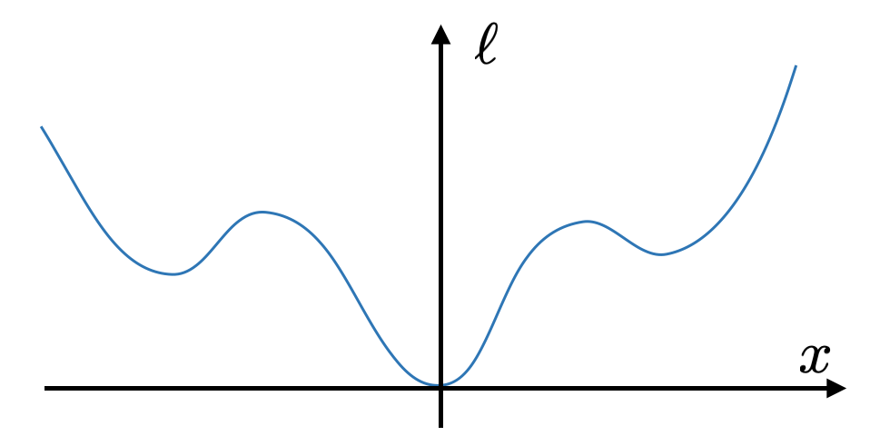
Control-Lyapunov Function for a Wheeled Robot
In this exercise, we examine the idea of a control-Lyapunov function
to drive a wheeled robot, implementing the controller proposed in
Similar to this previous
example, we use a kinematic model of the robot. We represent with
$z_1$ and $z_2$ its Cartesian position and with $z_3$ its orientation.
The controls are the linear $u_1$ and angular $u_2$ velocities. The
equations of motion read \begin{align*} \dot z_1 &= u_1 \cos z_3, \\ \dot
z_2 &= u_1 \sin z_3, \\ \dot z_3 &= u_2.\end{align*} The goal is to
design a feedback law $\pi(\bz)$ that drives the robot to the origin
$\bz=0$ from any initial condition. As pointed out in

- For the candidate Lyapunov function $V(\bx) = V_1(x_1) + V_2(x_2, x_3)$, with $V_1(x_1) = \frac{1}{2} x_1^2$ and $V_2(x_2, x_3) = \frac{1}{2}(x_2^2 + x_3^2)$, compute the time derivatives $\dot V_1 (\bx, u_1)$ and $\dot V_2(\bx, \bu)$.
- Show that the choice \begin{align*} u_1 &= \pi_1(\bx) = - x_1 \cos x_3, \\ u_2 &= \pi_2(\bx) = x_3 + \frac{(x_2 + x_3) \cos x_3 \sin x_3}{x_3}, \end{align*} makes $\dot V_1 (\bx, \pi_1(\bx)) \leq 0$ and $\dot V_2 (\bx, \pi(\bx)) \leq 0$ for all $\bx$. (Technically speaking, $\pi_2(\bx)$ is not defined for $x_3=0$. In this case, we let $\pi_2(\bx)$ assume its limiting value $x_2 + 2 x_3$, ensuring continuity of the feedback law.)
- Explain why Lyapunov's direct method does not allow us to establish asymptotic stability of the closed-loop system.
- Substitute the control law $\bu = \pi (\bx)$ in the equations of motion, and derive the closed-loop dynamics $\dot \bx = f(\bx, \pi(\bx))$. Use LaSalle's theorem to show (global) asymptotic stability of the closed-loop system.
- In we set up a simulation environment for you to try the controller we just derived. Type the control law from point (b) in the dedicated cell, and use the notebook plot to check your work.
SOS Polynomials in Lyapunov Analysis
- For each of the following polynomials, using
,
find whether they (1) admit a sum of squares formulation, and (2) are
positive semi-definite functions:
- $f_1(x) = x^2y^4 + x^4y^2 + 1 - 3x^2y^2$
- $f_2(x) = x^4 + 3y^4 - 2xy^3$
- $f_3(x, y, z; \lambda) = z^6 + x^2y^2(x^2 + y^2 - 3\lambda z^2)$, where $0 < \lambda \le 1$.
- If a fixed point of our dynamical system does not admit a SOS Lyapunov function, what can we conclude about its stability?
- If the optimal cost-to-go for a given dynamical system is not representable as sum of squares, can there still exist a SOS Lyapunov function? If no, explain why; otherwise, give an example of such a system.
ROA Estimation for the Time-Reversed Van der Pol Oscillator
In this exercise you will use SOS optimization to approximate the ROA of the time-reversed Van der Pol oscillator (a variation of the classical Van der Pol oscillator which evolves backwards in time). In , you are asked to test the following SOS formulations.
- The one from the example above, augmented with a line search that maximizes the area of the ROA.
- A single-shot SOS program that can directly maximize the area of the ROA, without any line search.
- An improved version of the previous, where less SOS constraints are imposed in the optimization problem.
Lyapunov Analysis for Robustness of Pendulum Swing-up Controllers
In this problem, we examine the robustness of the swing-up controller designed for the pendulum in this example using Lyapunov analysis. We consider an undamped pendulum in part (a)-(d), and one with damping ratio $b \neq 0$ in (e). Assume (1) we can measure $\theta$ and $\widetilde{\theta}$ perfectly (2) the pendulum does not start and will not stay at the downright position at any time.
- Suppose we have perfect measurements of mass $m$, length $l$, and the gravitational constant $g$. Show that the fixed point is attractive using LaSalle's Theorem and the scalar function $V(x)$.
- The swing-up controller is robust with respect to mass measurement. Suppose the mass measurement is incorrect $m_i \neq m$. Show that the controller can still complete the swing-up task, i.e., the fixed point is still attractive.
- Consider the case where both mass and length measurements are incorrect, $l_i \neq l$ and $m_i \neq m$. Is the fixed point still attractive? If not, identify conditions $m_i, l_i, \dot{\theta}, \theta, \widetilde{E}$ could satisfy such that $\dot{V} > 0$.
- Suppose in addition to uncertaint mass and length, the gravitational constant is also uncertain, $g_i \neq g$. Suppose the pendulum's small-oscillation period $T = 2\pi\sqrt{\frac{l}{g}}$ can be measured precisely, and the estimated values of length and gravitational constant satisfy $T = 2\pi\sqrt{\frac{l_i}{g_i}}$. Show that the controller can still complete the swing-up task, i.e., the fixed point is still attractive.
- Suppose we have accurate measurements of mass and length, but now the pendulum is damped, i.e., $b \neq 0$, and we have incorrect estimates of the damping ratio $b_i \neq b$. Using a swing-up controller $u = -k\dot{\theta}\widetilde{E} + b_i \dot{\theta}$, show that $V(x) = \frac{1}{2}\widetilde{E}^2$ cannot be used as a Lyapunov function to certify attractivity.