Multi-Body Dynamics
Deriving the equations of motion
The equations of motion for a standard robot can be derived using the method of Lagrange. Using $T$ as the total kinetic energy of the system, and $U$ as the total potential energy of the system, $L = T-U$, and $\tau_i$ as the element of the generalized force vector corresponding to $q_i$, the Lagrangian dynamic equations are: \begin{equation} \frac{d}{dt}\pd{L}{\dot{q}_i} - \pd{L}{q_i} = \tau_i.\end{equation} You can think of them as a generalization of Newton's equations. For a particle, we have $T=\frac{1}{2}m \dot{x}^2,$ so $\frac{d}{dt}\pd{L}{\dot{x}} = m\ddot{x},$ and $\pd{L}{x} = -\pd{U}{x} = f$ amounting to $f=ma$. But the Lagrangian derivation works in generalized coordinate systems and for constrained motion.
Simple Double Pendulum

Consider the simple double pendulum with torque actuation at both
joints and all of the mass concentrated in two points (for simplicity).
Using $\bq = [\theta_1,\theta_2]^T$, and ${\bf p}_1,{\bf p}_2$ to denote
the locations of $m_1,m_2$, respectively, the kinematics of this system
are:
\begin{eqnarray*}
{\bf p}_1 =& l_1\begin{bmatrix} s_1 \\ - c_1 \end{bmatrix}, &{\bf p}_2 =
{\bf p}_1 + l_2\begin{bmatrix} s_{1+2} \\ - c_{1+2} \end{bmatrix} \\
\dot{{\bf p}}_1 =& l_1 \dot{q}_1\begin{bmatrix} c_1 \\ s_1 \end{bmatrix},
&\dot{{\bf p}}_2 = \dot{{\bf p}}_1 + l_2 (\dot{q}_1+\dot{q}_2) \begin{bmatrix} c_{1+2} \\ s_{1+2} \end{bmatrix}
\end{eqnarray*}
Note that $s_1$ is shorthand for $\sin(q_1)$, $c_{1+2}$ is shorthand for
$\cos(q_1+q_2)$, etc. From this we can write the kinetic and potential
energy:
\begin{align*}
T =& \frac{1}{2} m_1 \dot{\bf p}_1^T \dot{\bf p}_1 + \frac{1}{2} m_2
\dot{\bf p}_2^T \dot{\bf p}_2 \\
=& \frac{1}{2}(m_1 + m_2) l_1^2 \dot{q}_1^2 + \frac{1}{2} m_2 l_2^2 (\dot{q}_1 + \dot{q}_2)^2 + m_2 l_1 l_2 \dot{q}_1 (\dot{q}_1 + \dot{q}_2) c_2 \\
U =& m_1 g y_1 + m_2 g y_2 = -(m_1+m_2) g l_1 c_1 - m_2 g l_2 c_{1+2}
\end{align*}
Taking the partial derivatives
\begin{align*}
\pd{T}{q_1} &= 0, \\
\pd{U}{q_1} & = (m_1 + m_2)gl_1s_1 + m_2 g l_2 s_{1+2}, \\
\pd{T}{q_2} &= - m_2 l_1 l_2 \dot{q}_1(\dot{q}_1 + \dot{q}_2)s_2, \\
\pd{U}{q_2} &= m_2 g l_2 s_{1+2}, \\
\pd{T}{\dot{q}_1} &= (m_1 + m_2) l_1^2 \dot{q}_1 + m_2 l_2^2 (\dot{q}_1 + \dot{q}_2) + m_2 l_1 l_2 (2 \dot{q}_1 + \dot{q}_2) c_2, \\
\pd{T}{\dot{q}_2} &= m_2 l_2^2 (\dot{q}_1 + \dot{q}_2) + m_2 l_1 l_2 \dot{q}_1 c_2, \\
\frac{d}{dt}\pd{T}{\dot{q}_1} &= (m_1+m_2)l_1^2 \ddot{q}_1 + m_2 l_2^2(\ddot{q}_1 + \ddot{q}_2) + m_2 l_1 l_2 (2 \ddot{q}_1 + \ddot{q}_2) c_2 - m_2 l_1 l_2 (2 \dot{q}_1 + \dot{q}_2) \dot{q}_2 s_2, \\
\frac{d}{dt}\pd{T}{\dot{q}_2} &= m_2 l_2^2 (\ddot{q}_1 + \ddot{q}_2) + m_2 l_1 l_2 \ddot{q}_1 c_2 - m_2 l_1 l_2 \dot{q}_1 \dot{q}_2 s_2,
\end{align*}
and plugging them into the Lagrangian, reveals the equations of motion:
\begin{align*}
(m_1 + m_2) l_1^2 \ddot{q}_1& + m_2 l_2^2 (\ddot{q}_1 + \ddot{q}_2) + m_2 l_1 l_2 (2 \ddot{q}_1 + \ddot{q}_2) c_2 \\
&- m_2 l_1 l_2 (2 \dot{q}_1 + \dot{q}_2) \dot{q}_2 s_2 + (m_1 + m_2) l_1 g s_1 + m_2 g l_2 s_{1+2} = \tau_1 \\
m_2 l_2^2 (\ddot{q}_1 + \ddot{q}_2)& + m_2 l_1 l_2 \ddot{q}_1 c_2 + m_2 l_1 l_2
\dot{q}_1^2 s_2 + m_2 g l_2 s_{1+2} = \tau_2
\end{align*}
As we saw in chapter 1, numerically integrating (and animating) these
equations in
If you are not comfortable with these equations, then any good book
chapter on rigid body mechanics can bring you up to speed.
I've also included a few more details about the connections between these equations and the variational principles of mechanics in the notes below, to the extent they may prove useful in our quest to write better optimizations for mechanical systems.
The Manipulator Equations
If you crank through the Lagrangian dynamics for a few simple robotic
manipulators, you will begin to see a pattern emerge - the resulting
equations of motion all have a characteristic form. For example, the
kinetic energy of your robot can always be written in the form:
\begin{equation} T = \frac{1}{2} \dot{\bq}^T \bM(\bq)
\dot{\bq},\end{equation} where $\bM$ is the state-dependent inertia matrix
(aka mass matrix). This observation affords some insight into general
manipulator dynamics - for example we know that ${\bf M}$ is always
positive definite, and symmetric
Continuing our abstractions, we find that the equations of motion of a general robotic manipulator (without kinematic loops) take the form \begin{equation}{\bf M}(\bq)\ddot{\bq} + \bC(\bq,\dot{\bq})\dot{\bq} = \btau_g(\bq) + {\bf B}\bu, \label{eq:manip} \end{equation} where $\bq$ is the joint position vector, ${\bf M}$ is the inertia matrix, $\bC$ captures Coriolis forces, and $\btau_g$ is the gravity vector. The matrix $\bB$ maps control inputs $\bu$ into generalized forces. Note that we pair $\bM\ddot\bq + \bC\dot\bq$ together on the left side because these terms together represent the force of inertia; the contribution from kinetic energy to the Lagrangian: $$\frac{d}{dt}\pd{T}{\dot{\bq}}^T - \pd{T}{\bq}^T = \bM(\bq) \ddot{\bq} + \bC(\bq,\dot\bq)\dot\bq.$$ Whenever I write Eq. (\ref{eq:manip}), I see $ma = f$.
Manipulator Equation form of the Simple Double Pendulum
The equations of motion from Example 1 can be written compactly as: \begin{align*} \bM(\bq) =& \begin{bmatrix} (m_1 + m_2)l_1^2 + m_2 l_2^2 + 2 m_2 l_1l_2 c_2 & m_2 l_2^2 + m_2 l_1 l_2 c_2 \\ m_2 l_2^2 + m_2 l_1 l_2 c_2 & m_2 l_2^2 \end{bmatrix} \\ \bC(\bq,\dot\bq) =& \begin{bmatrix} 0 & -m_2 l_1 l_2 (2\dot{q}_1 + \dot{q}_2)s_2 \\ \frac{1}{2} m_2 l_1 l_2 (2\dot{q}_1 + \dot{q}_2) s_2 & -\frac{1}{2}m_2 l_1 l_2 \dot{q}_1 s_2 \end{bmatrix} \\ \btau_g(\bq) =& -g \begin{bmatrix} (m_1 + m_2) l_1 s_1 + m_2 l_2 s_{1+2} \\ m_2 l_2 s_{1+2} \end{bmatrix} , \quad \bB = \begin{bmatrix} 1 & 0 \\ 0 & 1 \end{bmatrix} \end{align*} Note that this choice of the $\bC$ matrix was not unique. The manipulator equations are very general, but they do define some
important characteristics. For example, $\ddot{\bq}$ is (state-dependent)
linearly related to the control input, $\bu$. This observation justifies
the control-affine form of the dynamics assumed throughout the notes. There
are many other important properties that might prove useful. For instance,
we know that the $i$ element of $\bC\dot{\bq}$ is given by
Note that we have chosen to use the notation of second-order systems
(with $\dot{\bq}$ and $\ddot{\bq}$ appearing in the equations) throughout
this book. Although I believe it provides more clarity, there is an
important limitation to this notation: it is impossible to describe 3D
rotations in "minimal coordinates" using this notation without introducing
kinematic singularities (like the famous "gimbal lock"). For instance, a
common singularity-free choice for representing a 3D rotation is the unit
quaternion, described by 4 real values (plus a norm constraint). However
we can still represent the rotational velocity without singularities using
just 3 real values. This means that the length of our velocity vector is
no longer the same as the length of our position vector. For this reason,
you will see that most of the software in
Recursive Dynamics Algorithms
The equations of motions for our machines get complicated quickly.
Fortunately, for robots with a tree-link kinematic structure, there are
very efficient and natural recursive algorithms for generating these
equations of motion. For a detailed reference on these methods, see
Bilateral Position Constraints
If our robot has closed-kinematic chains, for instance those that arise from a four-bar linkage, then we need a little more. The Lagrangian machinery above assumes "minimal coordinates"; if our state vector $\bq$ contains all of the links in the kinematic chain, then we do not have a minimal parameterization -- each kinematic loop adds (at least) one constraint so should remove (at least) one degree of freedom. Although some constraints can be solved away, the more general solution is to use the Lagrangian to derive the dynamics of the unconstrained system (a kinematic tree without the closed-loop constraints), then add additional generalized forces that ensure that the constraint is always satisfied.
Consider the constraint equation \begin{equation}\bh(\bq) = 0.\end{equation} For example, in the case of the kinematic closed-chain, this can be the kinematic constraint that the location of one end of the chain is equal to the location of the other end of the chain. In the following derivation, we'll be using the time derivatives of this constraint: \begin{gather}\dot\bh = \bH\bv = 0,\\ \ddot\bh = \bH \dot\bv + \dot\bH \bv = 0, \label{eq:ddoth} \end{gather} where $\bH(\bq) = \pd{\bh}{\bq}{\bf N}(\bq)$ is the "Jacobian with respect to $\bv$". Note that $\dot{\bH}\bv$ is best calculated directly (rather than trying to solve for $\dot{\bH}$ as an object by itself).
The equations of motion can be written \begin{equation}\bM({\bq})\dot{\bv} + \bC(\bq,\bv)\bv = \btau_g(\bq) + \bB\bu + \bH^T(\bq) \blambda,\label{eq:constrained_manip}\end{equation} where ${\blambda}$ is the constraint force. Let's use the shorthand \begin{equation} \bM({\bq})\dot{\bv} = \btau(\bq,\dot{\bq},\bu) + \bH^T(\bq) \blambda. \label{eq:manip_short} \end{equation} In an optimization-based formulation (for instance, to implement this constraint in a trajectory optimization), we can simply make $\blambda$ a decision variable, and use equations (\ref{eq:ddoth}) and (\ref{eq:manip_short}) as constraints.
In other cases, it can be desirable to solve explicitly for $\blambda$. Inserting the dynamics (\ref{eq:manip_short}) into (\ref{eq:ddoth}) yields \begin{equation}\blambda =- (\bH \bM^{-1} \bH^T)^+ (\bH \bM^{-1} \btau + \dot\bH\bv).\label{eq:lambda_from_h}\end{equation} In many cases, this matrix will be full rank (for instance, in the case of multiple independent four-bar linkages) and the traditional inverse could have been used. When the matrix drops rank (multiple solutions), then the pseudo-inverse will select the solution with the smallest constraint forces in the least-squares sense.
To combat numerical "constraint drift", one might like to add a restoring force in the event that the constraint is not satisfied to numerical precision. To accomplish this, rather than solving for $\ddot\bh = 0$ as above, we can instead solve for \begin{equation}\ddot\bh = \bH\dot\bv + \dot\bH\bv = -2\alpha \dot\bh - \alpha^2 \bh,\end{equation} where $\alpha>0$ is a stiffness parameter. This is known as Baumgarte's stabilization technique, implemented here with a single parameter to provide a critically-damped response. Carrying this through yields \begin{equation} \blambda =- (\bH \bM^{-1} \bH^T)^+ (\bH \bM^{-1} \btau + \dot{\bH}\bv + 2\alpha \bH\bv + \alpha^2 \bh). \end{equation}
There is an important optimization-based derivation/interpretation of
these equations, which we will build on below, using Gauss's
Principle of Least Constraint. This principle says that we can
derive the constrained dynamics as : \begin{align} \min_\dot{\bv} \quad
& \frac{1}{2} (\dot{\bv} - \dot{\bv}_{uc})^T \bM (\dot{\bv} -
\dot{\bv}_{uc}), \label{eq:least_constraint} \\ \subjto \quad &
\ddot{\bh}(\bq,\bv,\dot\bv) = 0 = \bH \dot{\bv} + \dot\bH \bv,
\nonumber \end{align} where $\dot{\bv}_{uc} = \bM^{-1}\tau$ is the
"unconstrained acceleration"
Bilateral Velocity Constraints
Consider the constraint equation \begin{equation}\bh_v(\bq,\bv) = 0,\end{equation} where $\pd{\bh_v}{\bv} \ne 0.$ These are less common, but arise when, for instance, a joint is driven through a prescribed motion. Again, we will use the derivatives, \begin{equation} \dot\bh_v = \pd{\bh_v}{\bq} {\bf N}(\bq)\bv + \pd{\bh_v}{\bv}\dot{\bv} = 0,\label{eq:hvdot} \end{equation} and, the manipulator equations given by \begin{equation}\bM\dot{\bv} = \btau + \pd{\bh_v}{\bv}^T \blambda.\end{equation} These constraints can be added directly to an optimization with $\blambda$ as a decision variable. Alternatively, we can solve for $\blambda$ explicitly yielding \begin{equation}\blambda = - \left( \pd{\bh_v}{\bv} \bM^{-1} \pd{\bh_v}{\bv} \right)^+ \left[ \pd{\bh_v}{\bv} \bM^{-1} \btau + \pd{\bh_v}{\bq} {\bf N}(\bq) \bv \right].\end{equation}
Again, to combat constraint drift, we can ask instead for $\dot\bh_v = -\alpha \bh_v$, which yields \begin{equation}\blambda = - \left( \pd{\bh_v}{\bv} \bM^{-1} \pd{\bh_v}{\bv} \right)^+ \left[ \pd{\bh_v}{\bv} \bM^{-1} \btau + \pd{\bh_v}{\bq} {\bf N}(\bq) \bv + \alpha \bh_v \right].\end{equation}
Joint locking
Consider the simple, but important, case of "locking" a joint (making a particular joint act as if it is welded in the current configuration). One could write this as a bilateral velocity constraint $${\bf h}_v(\bq,\bv) = v_i = 0.$$ Since $\pd{{\bf h}_v}{\bv} = {\bf e}_i,$ (the vector with $1$ in the $i$th element and zero everywhere else, equation (\ref{eq:hvdot}) reduces to $\dot{v}_i = 0$, and $\pd{\bh_v}{\bv}^T \blambda$ impacts the equation for $\dot{v}_i$ and \emph{only} the equation for $\dot{v}_i$. The resulting equations can be obtained by simply removing the terms associated with $v_i$ from the manipulator dynamics (and setting $\dot{v}_i = 0$).
Hybrid models via constraint forces
For hybrid models of contact, it can be useful to work with a description of the dynamics in the floating-base coordinates and solve for the contact forces which enforce the constraints in each mode. We'll define a mode by a list of pairs of contact geometries that are in contact, and even define whether each contact is in sticking contact (with zero relative tangential velocity) or sliding contact. We can ask our geometry engine to return the contact points on the bodies, ${}^A{\bf p}^{C_a}$ and ${}^B{\bf p}^{C_b},$ where $C_a$ is the contact point (or closest point to contact) in body $A$ and $C_b$ is the contact point (or closest point to contact) in body $B$. More generally, we will refer to $C_a$ and $C_b$ as contact frames with their origins at these points, their $z$-axis pointing out along the contact normal, and their $x-y$-axes chosen as an orthonormal basis orthogonal to the normal.
For each sticking contact, we have a bilateral position constraint of the form $${\bf h}_{A,B}(\bq) = {}^W{\bf p}^{C_a}_{C_a} - {}^W{\bf p}^{C_b}_{C_a} = 0.$$ We can assemble all of these constraints into a single bilateral constraint vector ${\bf h}(\bq) = 0,$ and use almost precisely the recipe above. Note that applying Baumgarte stabilization here would only stabilize in the normal direction, by definition the vector between the two points, which is consistent with having (only) a zero-velocity constraint in the tangential direction. For sliding contacts, we have just the scalar constraint, $${\bf h}_{A,B}(\bq) = {}^W{\bf p}^{C_a}_{C_{a;z}} - {}^W{\bf p}^{C_b}_{C_{a;z}} = 0,$$ which says that the distance is zero in the normal direction, plus a constraint the imposes maximum dissipation $${\bf \lambda}^{C_a}_{C_{a;x,y}} = -\mu {\bf \lambda}^{C_a}_{C_{a;z}}\frac{{}^W{\bf \text{v}}^{C_a}_{C_{a;x,y}}}{|{}^W{\bf \text{v}}^{C_a}_{C_{a;x,y}}|},$$ that can be accommodated when we solve for $\lambda$.
The Dynamics of Contact
The dynamics of multibody systems that make and break contact are closely related to the dynamics of constrained systems, but tend to be much more complex. In the simplest form, you can think of non-penetration as an inequality constraint: the signed distance between collision bodies must be non-negative. But, as we have seen in the chapters on walking, the transitions when these constraints become active correspond to collisions, and for systems with momentum they require some care. We'll also see that frictional contact adds its own challenges.
There are three main approaches used to modeling contact with "rigid" body systems: 1) rigid contact approximated with stiff compliant contact, 2) hybrid models with collision event detection, impulsive reset maps, and continuous (constrained) dynamics between collision events, and 3) rigid contact approximated with time-averaged forces (impulses) in a time-stepping scheme. Each modeling approach has advantages/disadvantages for different applications.
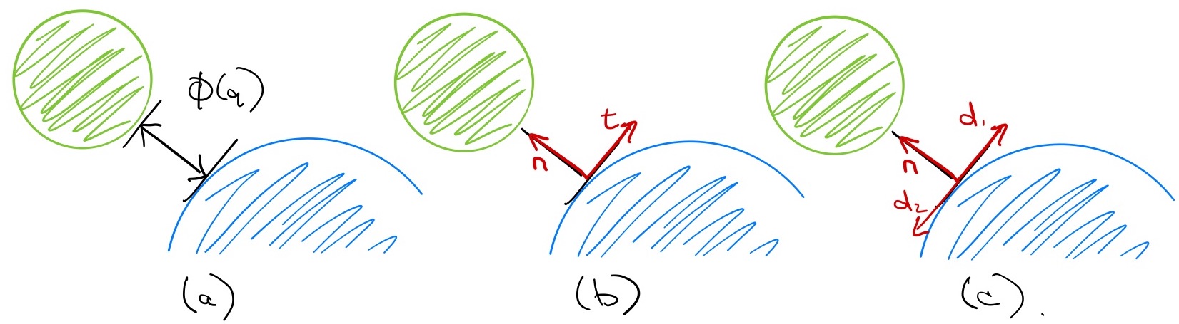
Before we begin, there is a bit of notation that we will use throughout. Let $\phi(\bq)$ indicate the relative (signed) distance between two rigid bodies. For rigid contact, we would like to enforce the unilateral constraint: \begin{equation} \phi(\bq) \geq 0. \end{equation} We'll use ${\bf n} = \pd{\phi}{\bq}$ to denote the "contact normal", as well as ${\bf t}_1$ and ${\bf t}_2$ as a basis for the tangents at the contact (orthonormal vectors in the Cartesian space, projected into joint space), all represented as row vectors in joint coordinates.
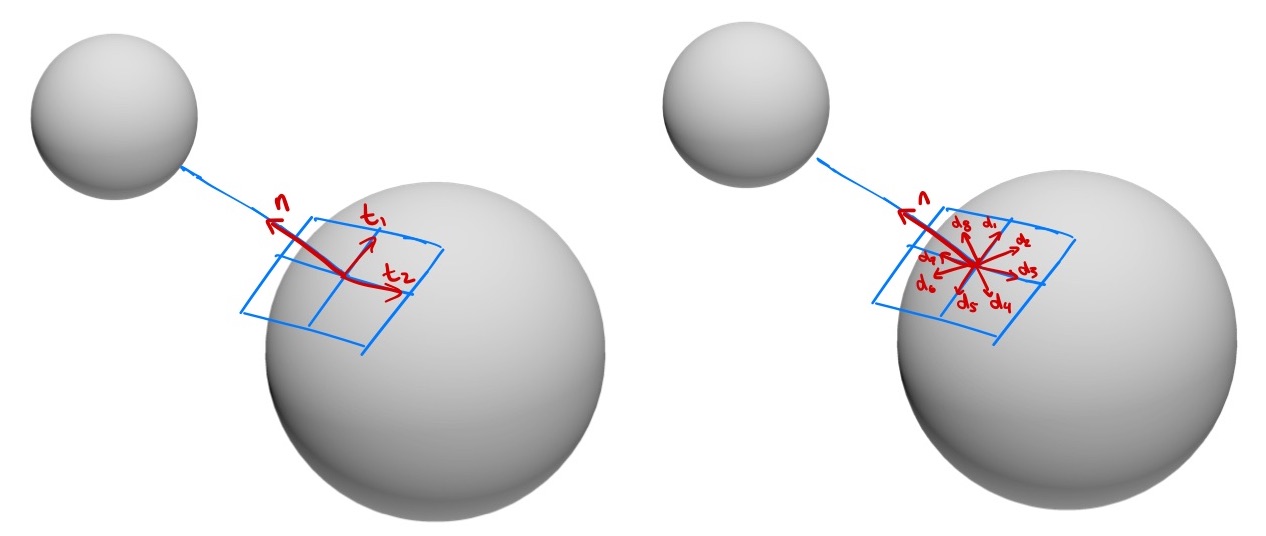
We will also find it useful to assemble the contact normal and tangent vectors into a single matrix, $\bJ$, that we'll call the contact Jacobian: $$\bJ(\bq) = \begin{bmatrix} {\bf n}\\ {\bf t}_1\\ {\bf t}_2 \end{bmatrix}.$$ As written, $\bJ\bv$ gives the relative velocity of the closest points in the contact coordinates; it can be also be extended with three more rows to output a full spatial velocity (e.g. when modeling torsional friction). The generalized force produced by the contact is given by $\bJ^T \lambda$, where $\lambda = [f_n, f_{t1}, f_{t2}]^T:$ \begin{equation} \bM(\bq) \dot{\bv} + \bC(\bq,\bv)\bv = \btau_g(\bq) + \bB \bu + \bJ^T(\bq)\lambda. \end{equation}
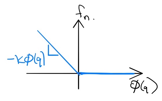
Compliant Contact Models
Most compliant contact models are conceptually straight-forward: we
will implement contact forces using a stiff spring (and
damper
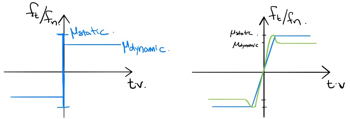
Coulomb friction is described by two parameters -- $\mu_{static}$ and $\mu_{dynamic}$ -- which are the coefficients of static and dynamic friction. When the contact tangential velocity (given by ${\bf t}\bv$) is zero, then friction will produce whatever force is necessary to resist motion, up to the threshold $\mu_{static} f_n.$ But once this threshold is exceeding, we have slip (non-zero contact tangential velocity); during slip friction will produce a constant drag force $|f_t| = \mu_{dynamic} f_n$ in the direction opposing the motion. This behavior is not a simple function of the current state, but we can approximate it with a continuous function as pictured below.
With these two laws, we can recover the contact forces as relatively simple functions of the current state. However, the devil is in the details. There are a few features of this approach that can make it numerically unstable. If you've ever been working in a robotics simulator and watched your robot take a step only to explode out of the ground and go flying through the air, you know what I mean.
In order to tightly approximate the (nearly) rigid contact that most
robots make with the world, the stiffness of the contact "springs" must be
quite high. For instance, I might want my 180kg humanoid robot model to
penetrate into the ground no more than 1mm during steady-state standing.
The challenge with adding stiff springs to our model is that this results
in stiff
differential equations (it is not a coincidence that the word
stiff is the common term for this in both springs and ODEs). As a
result, the best implementations of compliant contact for simulation make
use of special-purpose numerical integration recipes (e.g.
Note that there is one other type of friction that we talk about in robotics. In joints we also, additionally, model joint damping, often as a linear force proportional to the velocity which resists motion. Phenomenologically, this is due to a viscous (fluid) drag force produced by lubricants in the joint. The static and dynamic friction described above are sometimes collectively referred to as "dry" friction.
But there is another serious numerical challenge with the basic implementation of this model. Computing the signed-distance function, $\phi(\bq)$, when it is non-negative is straightforward, but robustly computing the "penetration depth" once two bodies are in collision is not. Consider the case of use $\bphi(\bq)$ to represent the maximum penetration depth of, say, two boxes that are contacting each other. With compliant contact, we must have some penetration to produce any contact force. But the direction of the normal vector, ${\bf n} = \pd{\bphi}{\bq},$ can easily change discontinuously as the point of maximal penetration moves, as I've tried to illustrate here:
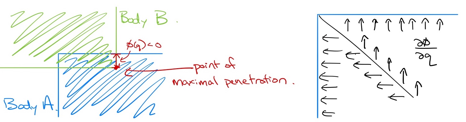
If you really think about this example, it actually reveals even more of the foibles of trying to even define the contact points and normals consistently. It seems reasonable to define the point on body B as the point of maximal penetration into body A, but notice that as I've drawn it, that isn't actually unique! The corresponding point on body A should probably be the point on the surface with the minimal distance from the max penetration point (other tempting choices would likely cause the distance to be discontinuous at the onset of penetration). But this whole strategy is asymmetric; why shouldn't I have picked the vector going with maximal penetration into body B? My point is simply that these cases exist, and that even our best software implementations get pretty unsatisfying when you look into the details. And in practice, it's a lot to expect the collision engine to give consistent and smooth contact points out in every situation.
Some of the advantages of this approach include (1) the fact that it is easy to implement, at least for simple geometries, (2) by virtue of being a continuous-time model it can be simulated with error-controlled integrators, and (3) the tightness of the approximation of "rigid" contact can be controlled through relatively intuitive parameters. However, the numerical challenges of dealing with penetration are very real, and they motivate our other two approaches that attempt to more strictly enforce the non-penetration constraints.
Rigid Contact with Event Detection
Impulsive Collisions
The collision event is described by the zero-crossings (from positive to negative) of $\phi$. Let us start by assuming frictionless collisions, allowing us to write \begin{equation}\bM\dot{\bv} = \btau + \lambda {\bf n}^T,\end{equation} where ${\bf n}$ is the "contact normal" we defined above and $\lambda \ge 0$ is now a (scalar) impulsive force that is well-defined when integrated over the time of the collision (denoted $t_c^-$ to $t_c^+$). Integrate both sides of the equation over that (instantaneous) interval: \begin{align*}\int_{t_c^-}^{t_c^+} dt\left[\bM \dot{\bv} \right] = \int_{t_c^-}^{t_c^+} dt \left[ \btau + \lambda {\bf n}^T \right] \end{align*} Since $\bM$, $\btau$, and ${\bf n}$ are constants over this interval, we are left with $$\bM{\bv}^+ - \bM{\bv}^- = {\bf n}^T \int_{t_c^-}^{t_c^+} \lambda dt,$$ where $\bv^+$ is short-hand for $\bv(t_c^+)$. Multiplying both sides by ${\bf n} \bM^{-1}$, we have $$ {\bf n} \bv^+ - {\bf n}\bv^- = {\bf n} \bM^{-1} {\bf n}^T \int_{t_c^-}^{t_c^+} \lambda dt.$$ After the collision, we have $\dot\phi^+ = -e \dot\phi^-$, with $0 \le e \le 1$ denoting the coefficient of restitution, yielding: $$ {\bf n} \bv^+ - {\bf n}\bv^- = -(1+e){\bf n}\bv^-,$$ and therefore $$\int_{t_c^-}^{t_c^+} \lambda dt = - (1+e)\left[ {\bf n} \bM^{-1} {\bf n}^T \right]^\# {\bf n} \bv^-.$$ I've used the notation $A^\#$ here to denote the pseudoinverse of $A$ (I would normally write $A^+,$ but have changed it for this section to avoid confusion). Substituting this back in above results in \begin{equation}\bv^+ = \left[ \bI - (1+e)\bM^{-1} {\bf n}^T \left[{\bf n} \bM^{-1} {\bf n}^T \right]^\# {\bf n} \right] \bv^-.\end{equation}
We can add friction at the contact. Rigid bodies will almost always
experience contact at only a point, so we typically ignore torsional
friction
A spinning ball bouncing on the ground.
Imagine a ball (a hollow-sphere) in the plane with mass $m$, radius $r$. The configuration is given by $q = \begin{bmatrix} x, z, \theta \end{bmatrix}^T.$ The equations of motion are $$\bM(\bq)\ddot\bq = \begin{bmatrix} m & 0 & 0 \\ 0 & m & 0 \\ 0 & 0 & \frac{2}{3}mr^2 \end{bmatrix} \ddot\bq = \begin{bmatrix} 0 \\ -g \\ 0 \end{bmatrix} + \begin{bmatrix} 0 & 1 \\ 1 & 0 \\ 0 & r \end{bmatrix} \begin{bmatrix} \lambda_z \\ \lambda_x \end{bmatrix} = \tau_g + \bJ^T {\bf \lambda},$$ where ${\bf \lambda}$ are the contact forces (which are zero except during the impulsive collision). Given a coefficient of restitution $e$ and a collision with a horizontal ground, the post-impact velocities are: $$ \dot{\bq}^+ = \begin{bmatrix} \frac{3}{5} & 0 & -\frac{2}{5} r \\ 0 & - e & 0 \\ -\frac{3}{5r} & 0 & \frac{2}{5}\end{bmatrix}\dot{\bq}^-.$$
Putting it all together
We can put the bilateral constraint equations and the impulsive collision equations together to implement a hybrid model for unilateral constraints of the form. Let us generalize \begin{equation}\bphi(\bq) \ge 0,\end{equation} to be the vector of all pairwise (signed) distance functions between rigid bodies; this vector describes all possible contacts. At every moment, some subset of the contacts are active, and can be treated as a bilateral constraint ($\bphi_i=0$). The guards of the hybrid model are when an inactive constraint becomes active ($\bphi_i>0 \rightarrow \bphi_i=0$), or when an active constraint becomes inactive ($\blambda_i>0 \rightarrow \blambda_i=0$ and $\dot\phi_i > 0$). Note that collision events will (almost always) only result in new active constraints when $e=0$, e.g. we have pure inelastic collisions, because elastic collisions will rarely permit sustained contact.
If the contact involves Coulomb friction, then the transitions between sticking and sliding can be modeled as additional hybrid guards.
Time-stepping Approximations for Rigid Contact
So far we have seen two different approaches to enforcing the inequality constraints of contact, $\phi(\bq) \ge 0$ and the friction cone. First we introduced compliant contact which effectively enforces non-penetration with a stiff spring. Then we discussed event detection as a means to switch between different models which treat the active constraints as equality constraints. But, perhaps surprisingly, one of the most popular and scalable approaches is something different: it involves formulating a mathematical program that can solve the inequality constraints directly on each time step of the simulation. These algorithms may be more expensive to compute on each time step, but they allow for stable simulations with potentially much larger and more consistent time steps.
Complementarity formulations
What class of mathematical program due we need to simulate contact?
The discrete nature of contact suggests that we might need some form of
combinatorial optimization. Indeed, the most common transcription is to
a Linear Complementarity Problem (LCP)
Rather than dive into the full transcription, which has many terms and can be relatively difficult to parse, let me start with two very simple examples.
Time-stepping LCP: Normal force
Consider our favorite simple mass being actuated by a horizontal force (with the double integrator dynamics), but this time we will add a wall that will prevent the cart position from taking negative values: our non-penetration constraint is $q \ge 0$. Physically, this constraint is implemented by a normal (horizontal) force, $f$, yielding the equations of motion: $$m\ddot{q} = u + f.$$
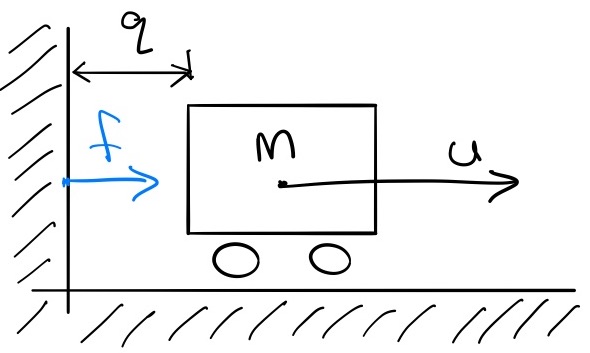
$f$ is defined as the force required to enforce the non-penetration constraint; certainly the following are true: $f \ge 0$ and $q \cdot f = 0$. $q \cdot f = 0$ is the "complementarity constraint", and you can read it here as "either q is zero or force is zero" (or both); it is our "no force at a distance" constraint, and it is clearly non-convex. It turns out that satisfying these constraints, plus $q \ge 0$, is sufficient to fully define $f$.
To define the LCP, we first discretize time, by approximating \begin{gather*}q[n+1] = q[n] + h v[n+1], \\ v[n+1] = v[n] + \frac{h}{m}(u[n] + f[n]).\end{gather*} This is almost the standard Euler approximation, but note the use of $v[n+1]$ in the right-hand side of the first equation -- this is actually a semi-implicit Euler approximation, and this choice is essential in the derivation.
Given $h, q[n], v[n],$ and $u[n]$, we can solve for $f[n]$ and $q[n+1]$ simultaneously, by solving the following LCP: \begin{gather*} q[n+1] = \left[ q[n] + h v[n] + \frac{h^2}{m} u[n] \right] + \frac{h^2}{m} f[n] \\ q[n+1] \ge 0, \quad f[n] \ge 0, \quad q[n+1]\cdot f[n] = 0. \end{gather*} Take a moment and convince yourself that this fits into the LCP prescription given above.
Note: Please don't confuse this visualization with the more common
visualization of the solution space for an LCP (in two or more
dimensions) in terms of "complementary cones"
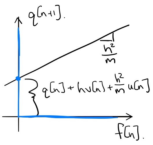
Perhaps it's also helpful to plot the solution, $q[n+1], f[n]$ as a function of $q[n], v[n]$. I've done it here for $m=1, h=0.1, u[n]=0$:
In the (time-stepping, "impulse-velocity") LCP formulation, we write the contact problem in it's combinatorial form. In the simple example above, the complementarity constraints force any solution to lie on either the positive x-axis ($f[n] \ge 0$) or the positive y-axis ($q[n+1] \ge 0$). The equality constraint is simply a line that will intersect with this constraint manifold at the solution. But in this frictionless case, it is important to realize that these are simply the optimality conditions of a convex optimization problem: the discrete-time version of Gauss's principle that we used above. Using $\bv'$ as shorthand for $\bv[n+1]$, and replacing $\ddot{\bq} = \frac{\bv' - \bv}{h}$ in Eq \eqref{eq:least_constraint} and scaling the objective by $h^2$ we have: \begin{align*} \min_{\bv'} \quad & \frac{1}{2} \left(\bv' - \bv - h\bM^{-1}\btau\right)^T \bM \left(\bv' - \bv - h\bM^{-1}\btau\right) \\ \subjto \quad & \frac{1}{h}\phi(\bq') = \frac{1}{h} \phi(\bq + h\bv') \approx \frac{1}{h}\phi(\bq) + {\bf n}\bv' \ge 0. \end{align*} The objective is even cleaner/more intuitive if we denote the next step velocity that would have occurred before the contact impulse is applied as $\bv^- = \bv + h\bM^{-1}\btau$: \begin{align*} \min_{\bv'} \quad & \frac{1}{2} \left(\bv' - \bv^-\right)^T \bM \left(\bv' - \bv^-\right) \\ \subjto \quad & \frac{1}{h}\phi(\bq') \ge 0. \end{align*} The LCP for the frictionless contact dynamics is precisely the optimality conditions of this convex (because $\bM \succeq 0$) quadratic program, and once again the contact impulse, ${\bf f} \ge 0$, plays the role of the Lagrange multiplier (with units $N\cdot s$).
So why do we talk so much about LCPs instead of QPs? Well LCPs can also represent a wider class of problems, which is what we arrive at with the standard transcription of Coulomb friction. In the limit of infinite friction, then we could add an additional constraint that the tangential velocity at each contact point was equal to zero (but these equation may not always have a feasible solution). Once we admit limits on the magnitude of the friction forces, the non-convexity of the disjunctive form rear's its ugly head.
Time-stepping LCP: Coulomb Friction
We can use LCP to find a feasible solution with Coulomb friction, but it requires some gymnastics with slack variables to make it work. For this case in particular, I believe a very simple example is best. Let's take our brick and remove the wall and the wheels (so we now have friction with the ground).
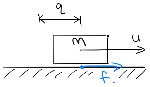
The dynamics are the same as our previous example, $$m\ddot{q} = u
+ f,$$ but this time I'm using $f$ for the friction force which is
inside the friction cone if $\dot{q} = 0$ and on the boundary of the
friction cone if $\dot{q} \ne 0;$ this is known as the principle of
maximum dissipation
Now, to write the friction constraints as an LCP, we must introduce some slack variables. First, we'll break the force into a positive component and a negative component: $f[n] = f^+ - f^-.$ And we will introduce one more variable $v_{abs}$ which will be non-zero if the velocity is non-zero (in either direction). Now we can write the LCP: \begin{align*} \find_{v_{abs}, f^+, f^-} \quad \subjto && \\ 0 \le v_{abs} + v[n+1] \quad &\perp& f^+ \ge 0, \\ 0 \le v_{abs} - v[n+1] \quad &\perp& f^- \ge 0, \\ 0 \le \mu mg - f^+ - f^- \quad &\perp& v_{abs} \ge 0,\end{align*} where each instance of $v[n+1]$ we write out with $$v[n+1] = v[n] + \frac{h}{m}(u + f^+ - f^-).$$ It's enough to make your head spin! But if you work it out, all of the constraints we want are there. For example, for $v[n+1] > 0$, then we must have $f^+=0$, $v_{abs} = v[n+1]$, and $f^- = \mu mg$. When $v[n+1] = 0$, we can have $v_{abs} = 0$, $f^+ - f^- \le \mu mg$, and those forces must add up to make $v[n+1] = 0$.
We can put it all together and write an LCP with both normal forces
and friction forces, related by Coulomb friction (using a polyhedral
approximation of the friction cone in 3d)
Anitescu's convex formulation
In
But be careful! Although the primal solution was convex, and the
dual problems are always convex, the objective here can be positive
semi-definite. This isn't a mistake --
When the tangential velocity is zero, this constraint is tight; for sliding contact the relaxation effectively causes the contact to "hydroplane" up out of contact, because $\phi(\bq') \ge h\mu {\bf d}_i\bv'.$ It seems like a quite reasonable approximation to me, especially for small $h$!
Let's continue on and write the dual program. To make the notation a little better, let us stack the Jacobian vectors into $\bJ_\beta$, such that the $i$th row is ${\bf n} + \mu{\bf d_i}$, so that we have $$\pd{L}{\bv'}^T = \bM(\bv' - \bv) - h\btau - \bJ_\beta^T \beta = 0.$$ Substituting this back into the Lagrangian give us the dual program: $$\min_{\beta \ge 0} \frac{1}{2} \beta^T \bJ_\beta \bM^{-1} \bJ_\beta^T \beta + \frac{1}{h}\phi(\bq) \sum_i \beta_i + \beta^T \bJ_\beta \bv^{-}.$$
One final note: I've written just one contact point here to simplify
the notation, but of course we repeat the constraint(s) for each contact
point;
Todorov's regularization
According to
How should we interpret this? If you expand the linear terms, you will see that this is almost exactly the dual form we get from the position equality constraints formulation, including the Baumgarte stabilization. It's interesting to think about the implications of this formulation -- like the Anitescu relaxation, it is possible to get some "force at a distance" because we have not in any way expressed that $\lambda = 0$ when $\phi(\bq) > 0.$ In Anitescu, it happened in a velocity-dependent boundary layer; here it could happen if you are "coming in hot" -- moving towards contact with enough relative velocity that the stabilization terms want to slow you down.
In dual form, it is natural to consider the full conic description of the friction cone: $$\mathcal{FC}(\bq) = \left\{{\bf \lambda} = [f_n, f_{t1}, f_{t2}]^T \middle| f_n \ge 0, \sqrt{f^2_{t1}+f^2_{t2}} \le \mu f_n \right\}.$$ The resulting dual optimization is has a quadratic objective and second-order cone constraints (SOCP).
There are a number of other important relaxations that happen in
MuJoCo. To address the positive indefiniteness in the objective,
The Semi-Analytic Primal (SAP) solver
The contact solver that we use in Drake further extends and improves upon this line of work...
Relaxed complementarity-free formulation: Normal force
What equations do we get if we simulate the simple cart colliding with a wall example that we used above?
Following
What remains is to compute $f[n]$, and here is where things get
interesting. Motivated by the idea of "softening the Gauss principle"
(e.g. the principle of least constraint
Beyond Point Contact
Coming soon... Box-on-plane example. Multi-contact.
Also a single point force cannot capture effects like torsional friction, and performs badly in some very simple cases (imaging a box sitting on a table). As a result, many of the most effective algorithms for contact restrict themselves to very limited/simplified geometry. For instance, one can place "point contacts" (zero-radius spheres) in the four corners of a robot's foot; in this case adding forces at exactly those four points as they penetrate some other body/mesh can give more consistent contact force locations/directions. A surprising number of simulators, especially for legged robots, do this.
In practice, most collision detection algorithms will return a list of "collision point pairs" given the list of bodies (with one point pair per pair of bodies in collision, or more if they are using the aforementioned "multi-contact" heuristics), and our contact force model simply attaches springs between these pairs. Given a point-pair, $p_A$ and $p_B$, both in world coordinates, ...
Hydroelastic model in drake
Variational mechanics
The field of analytic mechanics (or variational mechanics), has given us a number of different and potentially powerful interpretations of these equations. While our principle of virtual work was very much rooted in mechanical work, these variational principles have proven to be much more general. In the context of these notes, the variational principles also provide some deep connections between mechanics and optimization. So let's consider some of the equations above, but through the more general lens of variational mechanics.
Virtual work
Most of us are comfortable with the idea that a body is in equilibrium if the sum of all forces acting on that body (including gravity) is zero: $$\sum_i {\bf f}_i = 0.$$ It turns out that there are some limitations in working with forces directly: forces require us to (arbitrarily) define a coordinate system, and to achieve force balance we might need to consider all of the forces in the system, including internal forces like the forces at the joints that hold our robots together.
So it turns out to be better to think not about forces directly, but to think instead about the work, $w$, done by those forces. Work is force times distance. It's a scalar quantity, and it is invariant to the choice of coordinate system. Even for a system that is in equilibrium, we can reason about the virtual work that would occur if we were to make an infinitesimal change to the configuration of the system. Even better, since we know that the internal forces do no work, we can ignore them completely and only consider the virtual work that occurs due to a variation in the configuration variables. A multibody system in equilibrium must have zero virtual work: $$\delta w = \sum_i {\bf \tau}_i^T \delta \bq = 0.$$ Notice that these forces are the generalized forces (they have the same dimension as $\bq$). We can map between a Cartesian force and the generalized force using a kinematic Jacobian: ${\bf \tau}_i = {\bf J}_i^T(\bq){\bf f}_i.$ In particular, forces due to gravity, or any forces described by a "potential energy" function, are can be written as $${\bf \tau}_{g} = -\pd{U_{g}(\bq)}{\bq}^T.$$
If all of the generalized forces can be derived from such a potential function, then we can go even further. For a system to be in equilibrium, we must have that varations in the potential energy function must be zero, $\delta U(\bq) = 0.$ This follows simply from $\delta U = \pd{U}{\bq} \delta \bq$ and the principle of virtual work. Moreover, for the system to be in a stable equilibrium, $\bq$ must not only be a stationary point of the potential, but a minimum of the potential. This is our first important connection in this section between mechanics and optimization.
D'Alembert's principle and the force of inertia
What about bodies in motion? d'Alembert's principle states that we can reduce dynamics problems to statics problems by simply including a "force of inertia", which is the familiar mass times acceleration for simple particles. In order to have $\delta w = \sum_i {\bf \tau}_i^T \delta \bq = 0,$ for all $\delta \bq$, we must have $\sum_i {\bf \tau}_i = 0,$ so for multibody systems we know that the force of inertia must be: $${\bf \tau}_{inertia} = -{\bf M}(\bq)\ddot{\bq} - {\bf C}(\bq,\dot\bq)\dot{\bq}.$$ But where did that term come from? Is it the result of nature "optimizing" some scalar function?
A natural candidate would be the kinetic energy: $T(\bq, \dot\bq) = \frac{1}{2} \dot\bq^T {\bf M}(\bq) \dot\bq.$ What would it mean to take a variation of the kinetic energy, $\delta T?$ So far we've only had variations with respect to $\delta \bq$, but the kinetic energy depends on both $\bq$ and $\dot\bq$. We cannot vary these variables independently, but how are they related?
The solution is to take a variation not at a single point, but along a trajectory, where the relationship between $\delta \bq$ and $\delta \dot\bq$ is well defined. If we consider $$A(\bq(t)) = \int_{t_0}^{t_1} T(\bq,\dot\bq)dt,$$ then a variation of $A$ (using the calculus of variations) w.r.t. any trajectory $\bq(t)$, will take the form: $$\delta A = A(\bq(t) + \delta \bq(t)) - A(\bq(t) = \int_{t_0}^{t_1} T(\bq + \delta \bq(t), \dot\bq + \delta \dot\bq(t))dt - \int_{t_0}^{t_1} T(\bq(t), \dot\bq(t))dt,$$ where $\delta \bq(t)$ is defined to be an arbitrary (small) differentiable function in the space of $\bq$ that is zero at $t_0$ and $t_1.$
The derivation takes a few steps, which can be found in most mechanics texts. Click here to see my version.
We can expand the term in the first integral: $$T\left(\bq(t)+\bq(t),\, \dot\bq(t) + \delta \dot\bq(t)\right) = T\left(\bq(t),\,\dot\bq(t)\right) + \pd{T}{\bq(t)}\delta \bq(t) + \pd{T}{\dot\bq(t)}\delta \dot\bq(t).$$ Substituting this back in and simplifying leaves: $$\delta A = \int_{t_0}^{t_1} \left[\pd{T}{\bq(t)}\delta {\bf q}(t) + \pd{T}{\dot\bq(t)}\delta \dot{\bf q}(t)\right]dt.$$ Now use integration by parts on the second term: $$\int_{t_0}^{t_1} \pd{T}{\dot\bq(t)}\delta \dot{\bf q}(t)dt = \left[\pd{T}{\dot\bq(t)} \delta {\bf q}(t) \right]_{t_0}^{t_1} - \int_{t_0}^{t_1} \frac{d}{dt} \pd{T}{\dot\bq(t)} \delta {\bf q}(t) dt,$$ and observe that the first term in the right-hand side is zero since $\delta {\bf q}(t_0) = \delta {\bf q}(t_1) = 0$. This leaves $$\delta A = \int_{t_0}^{t_1} \left[\pd{T}{\bq} - \frac{d}{dt}\pd{T}{\dot\bq}\right]\delta {\bf q}(t) dt.$$ If our goal is to analyze the stationary points of this variation, then this quantity must integrate to zero for any ${\bf q}(t)$, so we must have $$\pd{T}{\bq} - \frac{d}{dt}\pd{T}{\dot\bq} = 0.$$
The result is that we find that the natural generalization of $-\pd{U(\bq)}{\bq}^T$ for stationary points of variations of quantities that also depend on velocity is $$\tau_{inertia} = -\pd{T}{\bq}^T + \frac{d}{dt}\pd{T}{\dot{\bq}}^T.$$ This is exactly (the negation of) our familiar $\bM(\bq) \ddot{\bq} + \bC(\bq,\dot\bq)\dot\bq.$
Principle of Stationary Action
The integral quantity $A$ that we used in the last section is commonly called the "action" of the system. More generally, the action is defined as $$A = \int_{t_0}^{t_1} L(\bq,\dot{\bq})dt,$$ where $L(\bq,\dot\bq)$ is an appropriate "Lagrangian" for the system. The Lagrangian has units of energy, but it is not uniquely defined. Any function which generates the correct equations of motion, in agreement with physical laws, can be taken as a Lagrangian. For our mechanical systems, the familiar form of the Lagrangian is what we presented above: $L = T - U$ (kinetic energy minus potential energy). Since the terms involving $U(\bq)$ do not depend directly on $\dot\bq$, they only contribute the $\pd{U}{\bq}^T$ terms that we expect, and taking $\delta A = 0$ for this Lagrangian is a way to generate the entire equations of motion in one go. For our purposes, where we care about conservative forces but also control inputs (as generalized forces $\bB \bu$), the principle of virtual work tells us that we will have $\delta A + \int_{t_0}^{t_1} \bu^T \bB^T \delta \bq(t) dt = 0.$
The viewpoint of variational mechanics is that it is this scalar
quantity $L(\bq,\dot\bq)$ that should be the central object of study (as
opposed to coordinate dependent forces), and this has proven to
generalize beautifully.
The principle of least action -- really the principle of stationary action -- is the most compact form of the classical laws of physics. This simple rule (it can be written in a single line) summarizes everything! Not only the principles of classical mechanics, but electromagnetism, general relativity, quantum mechanics, everything known about chemistry -- right down to the ultimate known constituents of matter, elementary particles.
Hamiltonian Mechanics
In some cases, it might be preferable to use the Hamiltonian formulation of the dynamics, with state variables $\bq$ and $\bp$ (instead of $\dot{\bq}$), where $\bp = \pd{L}{\dot{\bq}}^T = \bM \dot\bq$ results in the dynamics: \begin{align*}\bM(\bq) \dot{\bq} =& \bp \\ \dot{\bp} =& {\bf c}_H(\bq,\bp) + \tau_g(\bq) + \bB\bu, \qquad \text{where}\quad {\bf c}_H(\bq,\bp) = \frac{1}{2} \left(\pd{ \left[ \dot{\bq}^T \bM(\bq) \dot{\bq}\right]}{\bq}\right)^T.\end{align*} Recall that the Hamiltonian is $H({\bf p}, \bq) = {\bf p}^T\dot\bq - L(\bq,\dot\bq)$; these equations of motion are the familiar $\dot\bq = \pd{H}{\bf p}^T, \dot{\bf p} = -\pd{H}{\bq}^T.$
Exercises
Time-stepping LCP dynamics for block collision
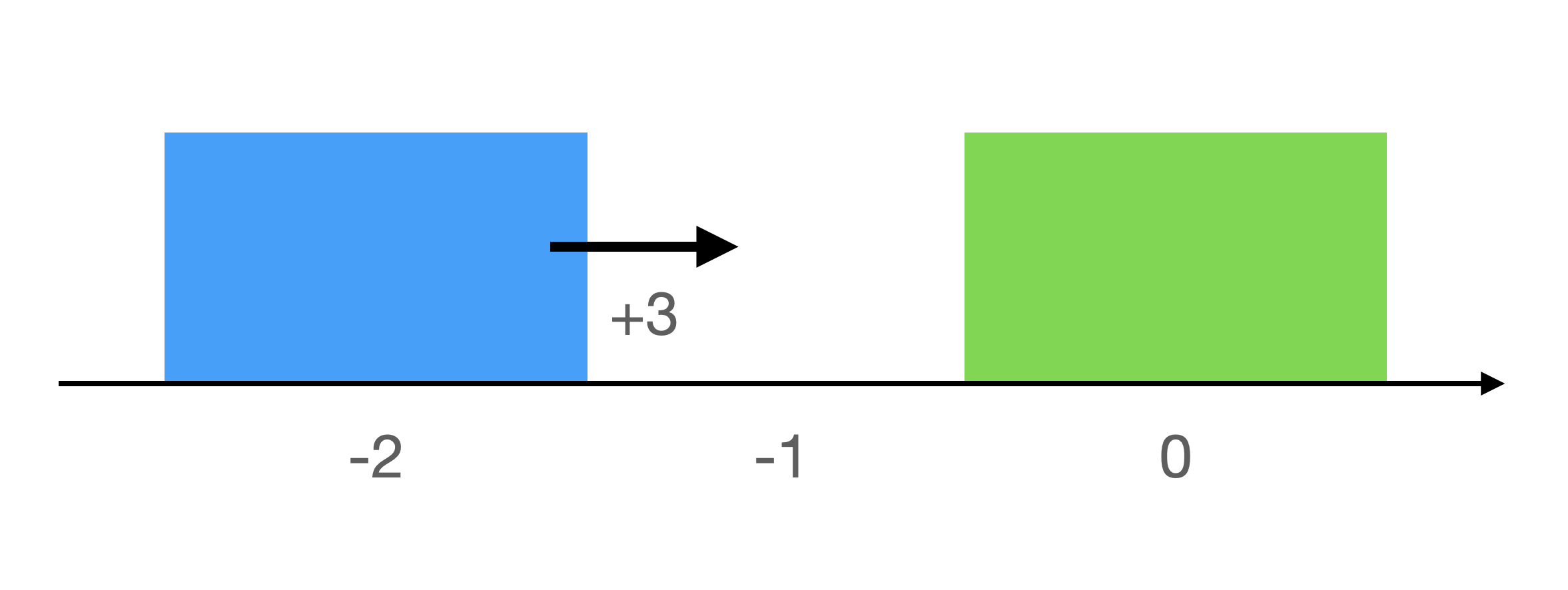
Suppose you have a block A of width 1, block B of width 1, interacting on a friction-less surface. The state of a single block in our system is $\vec{x} = \begin{bmatrix}q_x \\ \dot{q}_x \end{bmatrix}$, which represents the horizontal position (where the position point is located at the geometric center of the block) and horizontal velocity of the associated block. We have as our initial condition $\vec{x}^{(A)}_0 = \begin{bmatrix} -2 \\ 3 \end{bmatrix}$ and $\vec{x}^{(B)}_0 = \begin{bmatrix} 0 \\ 0 \end{bmatrix}$. In other words, at time step $0$ block A is moving towards a stationary block B located at the origin.
- Derive the positions, velocities, and contact forces at time steps 1, 2, and 3 for the two block collision scenario described at the start of this problem, under implicit Euler integration. Use time step $h=1.0$ and block masses $m_1 = m_2 = 1$.
Hint: See Example B.4 in the Appendix setting up the LCP optimization problem for a single cart and wall under semi-implicit integration. In implicit Euler integration, both the position and velocity are integrated with backward finite differences ($x[n+1] = x[n] + h f[n+1]$), whereas in the semi-implicit integration, only the position is integrated with backward finite differences.
Hint: To solve your LCP by hand, you should use the fact that time-stepping LCP produces perfectly inelastic collisions. What does the perfectly inelastic nature of collision imply about the signed distance during collision? - Since the block B is stationary, we might expect $q^{(A)}_{1, x} = -1$. Why is this not the case?
- What would you expect the velocities to be post-collision for perfectly inelastic collision and under conservation of momentum in continuous-time physics? How do these velocities compare with your time-stepped velocities?