Model-Free Policy Search
Reinforcement learning (RL) is a collection of algorithms for solving the same optimal control problem that we've focused on through the text, but the real gems from the RL literature are the algorithms for (almost) black-box optimization of stochastic optimal control problems. The idea of an algorithm that only has a "black-box" interface to the optimization problem means that it can obtain (potentially noisy) samples of the optimal cost via trial and error, but does not have access to the underlying model, and does not have direct access to complete gradient information.
This is a hard problem! In general we cannot expect RL algorithms to
optimize as quickly as more structured optimization, and we can typically only
guarantee convergence to a local optima at best. But the framework is
extremely general, so it can be applied to problems that are inaccessible to
any of the other algorithms we've examined so far. My favorite examples for
reinforcement learning are control in complex fluid dynamics (e.g.
In this chapter we will examine one particular style of reinforcement learning that attempts to find good controllers by explicitly parameterizing a family of policies (e.g. via a parameter vector $\alpha$), then searching directly for the parameters that optimize the long-term cost. For a stochastic optimal control problem with our favorite additive form of the objective, this might look like: \begin{equation} \min_\alpha E \left[ \sum_{n=0}^N \ell(\bx[n],\bu[n]) \right]\end{equation} where the random variables are drawn from probability densities \begin{gather*}\bx[0] \sim p_0(\bx),\\ \bx[n] \sim p(\bx[n] | \bx[n-1], \bu[n-1]), \\ \bu[n] \sim p_\alpha(\bu[n] | \bx[n]).\end{gather*} The last equation is a probabilistic representation of the control policy -- on each time-step actions $\bu$ are drawn from a distribution that is conditioned on the current state, $\bx$.
Of course, the controls community has investigated ideas like this, too, for instance under the umbrellas of extremum-seeking control and iterative learning control. I'll try to make connections whenever possible.
Policy Gradient Methods
One of the standard approaches to policy search in RL is to estimate the
gradient of the expected long-term cost with respect to the policy
parameters by evaluating some number of sample trajectories, then performing
(stochastic) gradient descent. Many of these so-called "policy gradient"
algorithms leverage a derivation called the likelihood ratio method
that was perhaps first described in
The Likelihood Ratio Method (aka REINFORCE)
Let's start with a simpler optimization over a stochastic function: $$\min_\alpha E\left[ g(\bx) \right] \text{ with } \bx \sim p_\alpha(\bx) $$ I hope the notation is clear? $\bx$ is a random vector, drawn from the distribution $p_\alpha(\bx)$, with the subscript indicating that the distribution depends on the parameter vector $\alpha$. What is the gradient of this function? The REINFORCE derivation is \begin{align*} \frac{\partial}{\partial \alpha} E \left[ g(\bx) \right] =& \frac{\partial}{\partial \alpha} \int d\bx ~ g(\bx) p_\alpha(\bx) \\ =& \int d\bx ~ g(\bx) \frac{\partial}{\partial \alpha} p_\alpha(\bx) \\ =& \int d\bx ~ g(\bx) p_\alpha(\bx) \frac{\partial}{\partial \alpha} \log p_\alpha(\bx) \\ =& E\left[ g(\bx) \frac{\partial}{\partial \alpha} \log p_\alpha(\bx) \right]. \end{align*} To achieve this, we used the derivative of the logarithm: \begin{gather*} y = \log u \\ \frac{\partial y}{\partial u} = \frac{1}{u} \frac{\partial u}{\partial x} \end{gather*} to write $$\frac{\partial}{\partial \alpha} p_\alpha(\bx) = p_\alpha(\bx) \frac{\partial}{\partial \alpha} \log p_\alpha(\bx).$$ This suggests a simple Monte Carlo algorithm for estimating the policy gradient: draw $N$ random samples $\bx_i$ then estimate the gradient as $$ \frac{\partial}{\partial \alpha} E \left[ g(\bx) \right] \approx \frac{1}{N} \sum_i g(\bx_i) \frac{\partial}{\partial \alpha} \log p_\alpha(\bx_i).$$
This trick is even more potent in the optimal control case. For a finite-horizon problem we have \begin{align*} \frac{\partial}{\partial \alpha} E \left[ \sum_{n=0}^N \ell(\bx[n], \bu[n]) \right] =& \int d\bx[\cdot] d\bu[\cdot] \left[ \sum_{n=0}^N \ell(\bx[n],\bu[n]) \right] \frac{\partial}{\partial \alpha} p_\alpha(\bx[\cdot], \bu[\cdot]) \\ =& E\left[ \left(\sum_{n=0}^N \ell(\bx[n],\bu[n])\right) \frac{\partial}{\partial \alpha} \log p_\alpha(\bx[\cdot],\bu[\cdot]) \right], \end{align*} where $\bx[\cdot]$ is shorthand for the entire trajectory $\bx[0], ..., \bx[N]$, and $$ p_\alpha(\bx[\cdot],\bu[\cdot]) = p_0(\bx[0]) \left(\prod_{k=1}^N p\left(\bx[k] \Big{|} \bx[k-1],\bu[k-1]\right) \right) \left(\prod_{k=0}^N p_\alpha(\bu[k] \Big{|} \bx[k]) \right).$$ Taking the $\log$ we have $$\log p_\alpha\left(\bx[\cdot],\bu[\cdot]\right) = \log p_0(\bx[0]) + \sum_{k=1}^N \log p(\bx[k] \Big{|} \bx[k-1],\bu[k-1]) + \sum_{k=0}^N \log p_\alpha(\bu[k] \Big{|} \bx[k]).$$ Only the last terms depend on $\alpha$, which yields \begin{align*} \frac{\partial}{\partial \alpha} E \left[ \sum_{n=0}^N \ell(\bx[n], \bu[n]) \right] &= E\left[ \left( \sum_{n=0}^N \ell(\bx[n],\bu[n]) \right) \left(\sum_{k=0}^N \frac{\partial}{\partial \alpha} \log p_\alpha\left(\bu[k]\Big{|}\bx[k]\right) \right) \right] \\ &= E\left[ \sum_{n=0}^N \left( \ell(\bx[n],\bu[n]) \sum_{k=0}^n \frac{\partial}{\partial \alpha} \log p_\alpha(\bu[k]\Big{|}\bx[k]) \right) \right], \end{align*} where the last step uses the fact that $E\left[\ell(\bx[n],\bu[n])\frac{\partial}{\partial \alpha} \log p_\alpha(\bu[k]\Big{|}\bx[k]) \right] = 0$ for all $k > n$.
This update should surprise you. It says that I can find the gradient of the long-term cost by taking only the gradient of the policy... but not the gradient of the plant, nor the cost! The intuition is that one can obtain the gradient by evaluating the policy along a number of (random) trajectory roll-outs of the closed-loop system, evaluating the cost on each, then increasing the probability in the policy of taking the actions correlated with lower long-term costs.
This derivation is often presented as the policy gradient derivation. The identity is certainly correct, but I'd prefer that you think of this as just one way to obtain the policy gradient. It's a particularly clever one in that it uses exactly the information that we have available in reinforcement learning -- we have access to the instantaneous costs, $\ell(\bx[n], \bu[n])$, and to the policy -- so are allowed to take gradients of the policy -- but does not require any understanding whatsoever of the plant model. Although it's clever, it is not particularly efficient -- the Monte Carlo approximations of the expected value have a high variance, so many samples are required for an accurate estimate. Other derivations are possible, some even simpler, and others that do make use of the plant gradients if you have access to them, and these will perform differently in the finite-sample approximations.
For the remainder of this section, I'd like to dig in and try to understand the nature of the stochastic update a little better, to help you understand what I mean.
Sample efficiency
Let's take a step back and think more generally about how one can use gradient descent in black-box (unconstrained) optimization. Imagine you have a simple optimization problem: $$\min_\alpha g(\alpha),$$ and you can directly evaluate $g()$, but not $\frac{\partial g}{\partial \alpha}$. How can you perform gradient descent?
A standard technique for estimating the gradients, in lieu of
analytical gradient information, is the method of finite
differences
What if each function evaluation is expensive? Perhaps it means picking up a physical robot and running it for 10 seconds for each evaluation of $g()$. Suddenly there is a premium on trying to optimize the cost function with the fewest number of evaluations on $g()$. This is the name of the game in reinforcement learning -- it's often called RL's sample complexity. Can we perform gradient descent using less evaluations?
Stochastic Gradient Descent
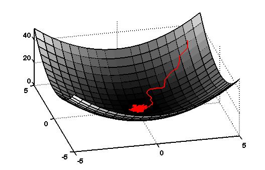
This leads us to the question of doing approximate gradient descent, or
"stochastic" gradient descent. Thinking of the cost landscape as a
Lyapunov function†
The Weight Pertubation Algorithm
Instead of sampling each dimension independently, consider making a single small random change, $\bbeta$, to the parameter vector, $\balpha$. Now consider the update of the form: $$\Delta \balpha= -\eta [ g(\balpha + \bbeta) - g(\balpha)]\bbeta.$$ The intuition here is that if $g(\balpha+\bbeta) < g(\balpha)$, then $\bbeta$ was a good change and we'll move in the direction of $\bbeta$. If the cost increased, then we'll move in the opposite direction. Assuming the function is smooth and $\bbeta$ is small, then we will always move downhill on the Lyapunov function.
Even more interesting, on average, the update is actually in the direction of the true gradient. To see this, again we can assume the function is locally smooth and $\bbeta$ is small to write the Taylor expansion: $$g(\balpha + \bbeta) \approx g(\balpha) + \pd{g}{\balpha}\bbeta.$$ Now we have \begin{align*}\Delta \balpha \approx& -\eta \left[ \pd{g}{\alpha} \bbeta \right] \bbeta = -\eta \bbeta \bbeta^T \pd{g}{\balpha}^T \\ \avg{\Delta \balpha} \approx& -\eta \avg{\bbeta \bbeta^T} \pd{g}{\balpha}^T \end{align*} If we select each element of $\bbeta$ independently from a distribution with zero mean and variance $\sigma_\beta^2$, or $\avg{ \beta_i } = 0, \avg{ \beta_i \beta_j } = \sigma_\beta^2 \delta_{ij}$, then we have $$\avg{\Delta \balpha} \approx -\eta \sigma_\beta^2 \pd{g}{\balpha}^T.$$ Note that the distribution $p_{\alpha}(\bx)$ need not be Gaussian, but it is the variance of the distribution which determines the scaling on the gradient.
Weight Perturbation with an Estimated Baseline
The weight perturbation update above requires us to evaluate the function $g$ twice for every update of the parameters. This is low compared to the method of finite differences, but let us see if we can do better. What if, instead of evaluating the function twice per update [$g(\balpha+\bbeta)$ and $g(\balpha)$], we replace the evaluation of $g(\balpha)$ with an estimator, $b = \hat{g}(\balpha)$, obtained from previous trials? In other words, consider an update of the form: \begin{equation} \Delta \balpha= - \frac{\eta}{\sigma_\beta^2} [ g(\balpha + \bbeta) - b]\bbeta \label{eq:weight_perturbation_baseline} \end{equation} The estimator can take any of a number of forms, but perhaps the simplest is based on the update (after the $n$th trial): $$b[n+1] = \gamma g[n] + (1 - \gamma)b[n],\quad b[0] = 0, 0\le\gamma\le1,$$ where $\gamma$ parameterizes the moving average. Let's compute the expected value of the update, using the same Taylor expansion that we used above: \begin{align*} E[\Delta \balpha] =& -\frac{\eta}{\sigma_\beta^2} \avg{ [g(\balpha) + \pd{g}{\balpha}\bbeta - b]\bbeta} \\ =& -\frac{\eta}{\sigma_\beta^2} \avg{[g(\balpha)-b]\bbeta} -\frac{\eta}{\sigma_\beta^2} \avg{\bbeta \bbeta^T}\pd{g}{\balpha}^T \\ =& - \eta \pd{g}{\balpha}^T \end{align*} In other words, the baseline does not effect our basic result - that the expected update is in the direction of the gradient. Note that this computation works for any baseline estimator which is uncorrelated with $\bbeta$, as it should be if the estimator is a function of the performance in previous trials.
Although using an estimated baseline doesn't effect the average update, it can have a dramatic effect on the performance of the algorithm. As we will see in a later section, if the evaluation of $g$ is stochastic, then the update with a baseline estimator can actually outperform an update using straight function evaluations.
Let's take the extreme case of $b=0$. This seems like a very bad idea... on each step we will move in the direction of every random perturbation, but we will move more or less in that direction based on the evaluated cost. In average, we will still move in the direction of the true gradient, but only because we will eventually move more downhill than we move uphill. It feels very naive.
REINFORCE w/ additive Gaussian noise
Now let's consider the simple form of the REINFORCE update: \begin{align*} \frac{\partial}{\partial \alpha} E \left[ g(\bx) \right] = E\left[ g(\bx) \frac{\partial}{\partial \alpha} \log p_\alpha(\bx) \right]. \end{align*} It turns out that weight perturbation is a REINFORCE algorithm. To see this, take $\bx = \balpha + \bbeta$, $\bbeta \in N(0,\sigma^2)$, to have \begin{gather*} p_{\balpha}(\bx) = \frac{1}{(2\pi\sigma^2)^N} e^{\frac{-(\bx-\balpha)^T(\bx - \balpha)}{2\sigma^2}} \\ \log p_{\balpha}(\bx) = \frac{-(\bx-\balpha)^T(\bx - \balpha)}{2\sigma^2} + \text{terms that don't depend on }\balpha \\ \pd{}{\balpha} \log p_{\balpha}(\bx) = \frac{1}{\sigma^2} (\balpha - \bx)^T = \frac{1}{\sigma^2} \bbeta^T. \\ \end{gather*} If we use only a single trial for each Monte-Carlo evaluation, then the REINFORCE update is $$\Delta \balpha = -\frac{\eta}{\sigma^2} g(\balpha + \bbeta) \bbeta,$$ which is precisely the weight perturbation update (the crazy version with $b=0$ discussed above). Although it will move in the direction of the gradient on average, it can be highly inefficient. In practice, people use many more than one sample to estimate the poilicy gradient.
Summary
The policy gradient "trick" from REINFORCE using log probabilities provides one means of estimating the true policy gradient. It is not the only way to obtain the policy gradient... in fact the trivial weight-perturbation update obtains the same gradient for the case of a policy with a mean linear in $\alpha$ and a fixed diagonal covariance. It's cleverness lies in the fact that it makes use of the information we do have (instantaneous cost values and the gradients of the policy), and that it provides an unbiased estimate of the gradient (note that taking the gradients of a model that is only slightly wrong might not have this virtue). But its inefficiency comes from having a potentially very high variance. Variance reduction for policy gradient, often through baseline estimation, continues to be an active area of research.
Sample performance via the signal-to-noise ratio.
Performance of Weight Perturbation
The simplicity of the REINFORCE / weight perturbation updates makes it tempting to apply them to problems of arbitrary complexity. But a major concern for the algorithm is its performance - although we have shown that the update is in the direction of the true gradient on average, it may still require a prohibitive number of computations to obtain a local minima.
In this section, we will investigate the performance of the weight
perturbation algorithm by investigating its signal-to-noise ratio
(SNR). This idea was explored in
For the weight perturbation update we have: $$\avg{\Delta \balpha}^T\avg{\Delta \balpha} = \eta^2 \pd{g}{\balpha} \pd{g}{\balpha}^T = \eta^2 \sum_{i=1}^{N} \left( \pd{g}{\alpha_i} \right)^2,$$ \begin{align*} \avg{(\Delta \balpha)^T(\Delta \balpha)} =& \frac{\eta^2}{\sigma_\beta^4} \avg{\left[g(\balpha+\bbeta) - g(\balpha)\right]^2 \bbeta^T\bbeta} \\ \approx& \frac{\eta^2}{\sigma_\beta^4} \avg{ \left[ \pd{g}{\balpha} \bbeta \right]^2 \bbeta^T\bbeta } \\ =& \frac{\eta^2}{\sigma_\beta^4} \avg{ \left(\sum_i \pd{g}{\alpha_i}\beta_i\right) \left( \sum_j \pd{g}{\alpha_j} \beta_j\right) \left(\sum_k \beta_k^2 \right) } \\ =& \frac{\eta^2}{\sigma_\beta^4} \avg{ \sum_i \pd{g}{\alpha_i}\beta_i \sum_j \pd{g}{\alpha_j} \beta_j \sum_k \beta_k^2 } \\ =& \frac{\eta^2}{\sigma_\beta^4} \sum_{i,j,k} \pd{g}{\alpha_i} \pd{g}{\alpha_j} \avg{ \beta_i \beta_j \beta_k^2 }\\ \avg{\beta_i \beta_j \beta_k^2} = \begin{cases} 0 & i \neq j \\ \sigma_\beta^4 & i=j\neq k \\ \mu_4(\beta) & i = j =k \end{cases}& \\ =& \eta^2 (N-1) \sum_i \left( \pd{g}{\alpha_i} \right)^2 + \frac{\eta^2 \mu_4(z)}{\sigma_\beta^4} \sum_i \left(\pd{g}{\alpha_i}\right)^2 \end{align*} where $\mu_n(z)$ is the $n$th central moment of $z$: $$\mu_n(z) = \avg{(z - \avg{z})^n}.$$ Putting it all together, we have: $$\text{SNR} = \frac{1}{N - 2 + \frac{\mu_4(\beta_i)}{\sigma_\beta^4}}.$$
Signal-to-noise ratio for additive Gaussian noise
For $\beta_i$ drawn from a Gaussian distribution, we have $\mu_1 = 0, \mu_2 = \sigma^2_\beta, \mu_3 = 0, \mu_4 = 3 \sigma^4_\beta,$ simplifying the above expression to: $$\text{SNR} = \frac{1}{N+1}.$$
Signal-to-noise ratio for additive uniform noise
For $\beta_i$ drawn from a uniform distribution over [-a,a], we have $\mu_1 = 0, \mu_2 = \frac{a^2}{3} = \sigma_\beta^2, \mu_3 = 0, \mu_4 = \frac{a^4}{5} = \frac{9}{5}\sigma_\beta^4,$ simplifying the above to: $$\text{SNR} = \frac{1}{N-\frac{1}{5}}.$$
Performance calculations using the SNR can be used to design the parameters of the algorithm in practice. For example, based on these results it is apparent that noise added through a uniform distribution yields better gradient estimates than the Gaussian noise case for very small $N$, but that these differences are neglibile for large $N$.
Similar calculations can yield insight into picking the size of the additive noise (scaled by $\sigma_\beta$). The calculations in this section seem to imply that larger $\sigma_\beta$ can only reduce the variance, overcoming errors or noise in the baseline estimator, $\tilde{b}$; this is a short-coming of our first-order Taylor expansion. If the cost function is not linear in the parameters, then an examination of higher-order terms reveals that large $\sigma_\beta$ can increase the SNR. The derivation with a second-order Taylor expansion is left for an exercise.