Trajectory Optimization
I've argued that optimal control is a powerful framework for specifying complex behaviors with simple objective functions, letting the dynamics and constraints on the system shape the resulting feedback controller (and vice versa!). But the computational tools that we've provided so far have been limited in some important ways. The numerical approaches to dynamic programming which involve putting a mesh over the state space do not scale well to systems with state dimension more than four or five. Linearization around a nominal operating point (or trajectory) allowed us to solve for locally optimal control policies (e.g. using LQR) for even very high-dimensional systems, but the effectiveness of the resulting controllers is limited to the region of state space where the linearization is a good approximation of the nonlinear dynamics. The computational tools for Lyapunov analysis from the last chapter can provide, among other things, an effective way to compute estimates of those regions, and the sums-of-squares approaches to dynamic programming are still in their early days. We have not yet provided the mainstream computational tools for approximate optimal control that work for high-dimensional systems beyond the linearization around a goal. That is precisely the goal for this chapter.
In order to scale to high-dimensional systems, we are going to formulate a simpler version of the optimization problem. Rather than trying to solve for the optimal feedback controller for the entire state space, in this chapter we will instead attempt to find an optimal control solution that is valid from only a single initial condition. Instead of representing this as a feedback control function, we can represent this solution as a trajectory, $\bx(t), \bu(t)$, typically defined over a finite interval.
Problem Formulation
Given a state-space model, $\dot{\bx} = f(\bx,\bu)$, an initial condition, $\bx_0$, and an input trajectory $\bu(t)$ defined over a finite interval, $t\in[t_0,t_f],$ we can simulate the dynamics forward to obtain $\bx(t)$ over the same interval. We will define the long-term (finite-horizon) cost of executing that trajectory using the standard additive-cost optimal control objective, \[ J_{\bu(\cdot)}(\bx_0) = \ell_f (\bx(t_f)) + \int_{t_0}^{t_f} \ell(\bx(t),\bu(t)) dt. \] $\ell_f$ is a terminal cost, evaluated at the end of the trajectory, which we did not have in the infinite-horizon formulations we've focused on so far. We will write the trajectory optimization problem as \begin{align*} \min_{\bu(\cdot)} \quad & \ell_f (\bx(t_f)) + \int_{t_0}^{t_f} \ell(\bx(t),\bu(t)) dt \\ \subjto \quad & \dot{\bx}(t) = f(\bx(t),\bu(t)), \quad \forall t\in[t_0, t_f] \\ & \bx(t_0) = \bx_0. \\ \end{align*} Many trajectory optimization problems will also include additional constraints, such as collision avoidance (e.g., where the constraint is that the signed distance between the robot's geometry and the obstacles stays positive) or input limits (e.g. $\bu_{min} \le \bu \le \bu_{max}$ ). Constraints can be defined for all time or some subset of the trajectory.
As written, the optimization above is an optimization over continuous
trajectories. In order to formulate this as a numerical optimization, we
must parameterize it with a finite set of numbers. Perhaps not
surprisingly, there are many different ways to write down this
parameterization, with a variety of different properties in terms of speed,
robustness, and accuracy of the results. We will outline just a few of the
most popular below; I would recommend
It is worth contrasting this parameterization problem with the one that we faced in our continuous-dynamic programming algorithms. For trajectory optimization, we need a finite-dimensional parameterization in only one dimension (time), whereas in the mesh-based value iteration algorithms we had to work in the dimension of the state space. Our mesh-based discretizations scaled badly with this state dimension, and led to numerical errors that were difficult to deal with. Discreting over just one dimension (time), is fundamentally different. There is relatively much more known about discretizing solutions to differential equations over time, including work on error-controlled integration. And the number of parameters required for trajectory parameterizations scales linearly with the state dimension, instead of exponentially in mesh-based value iteration.
Convex Formulations for Linear Systems
Let us first consider the case of linear systems. In fact, if we start in discrete time with a state space model of the form $\bx[n+1] = {\bf A}\bx[n] + {\bf B}\bu[n]$, we can even defer the question of how to best discretize the continuous-time problem. There are a few different ways that we might "transcribe" this optimization problem into a concrete mathematical program.
Direct Transcription
For instance, let us start by writing both $\bu[\cdot]$ and $\bx[\cdot]$ as decision variables. Then we can write: \begin{align*} \min_{\bx[\cdot],\bu[\cdot]} \quad & \ell_f(\bx[N]) + \sum_{n=0}^{N-1} \ell(\bx[n],\bu[n]) \\ \subjto \quad & \bx[n+1] = {\bf A}\bx[n] + {\bf B}\bu[n], \quad \forall n\in[0, N-1] \\ & \bx[0] = \bx_0 \\ & + \text{additional constraints}. \end{align*} We call this modeling choice -- adding $\bx[\cdot]$ as decision variables and modeling the discrete dynamics as explicit constraints -- the "direct transcription". Importantly, for linear systems, the dynamics constraints are linear constraints in these decision variables. As a result, if we can restrict our additional constraints to linear inequality constraints and our objective function to being linear/quadratic in $\bx$ and $\bu$, then the resulting trajectory optimization is a convex optimization (specifically a linear program or quadratic program depending on the objective). We can reliably solve these problems to global optimality at quite large scale; these days it is common to solve these optimization online inside a high-rate feedback controller.
Trajectory optimization for the Double Integrator
We've looked at a few optimal control problems for the double integrator using value iteration. For one of them -- the quadratic objective with no constraints on $\bu$ -- we know now that we could have solved the problem "exactly" using LQR. But we have not yet given satisfying numerical solutions for the minimum-time problem, nor for the constrained LQR problem.
In the trajectory formulation, we can solve these problems exactly for the discrete-time double integrator, and with better accuracy for the continuous-time double integrator. Take a moment to appreciate that! The bang-bang policy and cost-to-go functions are fairly nontrivial functions of state; it's quite satisfying that we can evaluate them using convex optimization! The limitation, of course, is that we are only solving them for one initial condition at a time.
If you have not studied convex optimization before, you might be surprised by the modeling power of even of this framework. Consider, for instance, an objective of the form $$\ell(\bx,\bu) = |\bx| + |\bu|.$$ This can be formulated as a linear program. To do it, add additional decision variables ${\bf s}_x[\cdot]$ and ${\bf s}_u[\cdot]$ -- these are commonly referred to as slack variables -- and write $$\min_{\bx,\bu,{\bf s}_x,{\bf s}_u} \sum_n^{N-1} {\bf s}_x[n] + {\bf s}_u[n], \quad \text{s.t.} \quad {\bf s}_x[n] \ge \bx[n], \quad {\bf s}_x[n] \ge -\bx[n], \quad ...$$ The field of convex optimization is replete with tricks like this. Knowing and recognizing them are skills of the (optimization) trade. But there are also many relevant constraints which cannot be recast into convex constraints (in the original coordinates) with any amount of skill. An important example is obstacle avoidance. Imagine a vehicle that must decide if it should go left or right around an obstacle. This represents a fundamentally non-convex constraint in $\bx$; we'll discuss the implications of using non-convex optimization for trajectory optimization below.
Direct Shooting
The savvy reader might have noticed that adding $\bx[\cdot]$ as decision variables was not strictly necessary. If we know $\bx[0]$ and we know $\bu[\cdot]$, then we should be able to solve for $\bx[n]$ using forward simulation. For our discrete-time linear systems, this is particularly nice: \begin{align*} \bx[1] =& \bA\bx[0] + \bB\bu[0] \\ \bx[2] =& \bA(\bA\bx[0] + \bB\bu[0]) + \bB\bu[1] \\ \bx[n] =& \bA^n\bx[0] + \sum_{k=0}^{n-1} \bA^{n-1-k}\bB\bu[k]. \end{align*} What's more, the solution is still linear in $\bu[\cdot]$. This is amazing... we can get rid of a bunch of decision variables, and turn a constrained optimization problem into an unconstrained optimization problem (assuming we don't have any other constraints). This approach -- using $\bu[\cdot]$ but not $\bx[\cdot]$ as decision variables and using forward simulation to obtain $\bx[n]$ -- is called the direct shooting transcription. For linear systems with linear/quadratic objectives in $\bx$, and $\bu$, it is still a convex optimization, and has less decision variables and constraints than the direct transcription.
Computational Considerations
So is direct shooting uniformly better than the direct transcription approach? I think it is not. There are a few potential reason that one might prefer the direct transcription:
- Numerical conditioning. Shooting involves calculating ${\bf A}^n$ for potentially large $n$, which can lead to a large range of coefficient values in the constraints. This problem is sometimes referred to as the "tail wagging the dog", or in very deep neural networks as "vanishing gradients" and/or "exploding gradients". In trajectory optimization, it is not simply an artifact of the shooting transcription, but is a real property of the problem we have formulated: the control input $\bu[0]$ really does have more opportunity to have a large impact on the total cost than control input $\bu[N-1]$. The direct transcription approach combats the numerical issue by spreading this effect out over a large number of well-balanced constraints.
- Adding state constraints. Having $\bx[n]$ as explicit decision variables makes it very easy/natural to add additional state constraints; and the solver effectively reuses the computation of ${\bf A}^n$ for each constraint. In shooting, one has to unroll those terms for each new constraint.
- Parallelization. For larger problems, evaluating the constraints can be a substantial cost. In direct transcription, one can evaluate the dynamics/constraints in parallel (because each iteration begins with $\bx[n]$ already given), whereas shooting is more fundamentally a serial operation.
For linear convex problems, the solvers are mature enough that these differences often don't amount to much. For nonlinear optimization problems, the differences can be substantial. If you look at trajectory optimization papers in mainstream robotics, you will see that both direct transcription and direct shooting approaches are used. (It used to be that you could guess which research lab wrote a paper simply by the transcription they use!)
It is also worth noting that the problems generated by the direct
transcription have an important and exploitable "banded" sparsity pattern
-- most of the constraints touch only a small number of variables. This
is actually the same pattern that we exploit in the Riccati equations.
Thanks to the importance of these methods in real applications, numerous
specialized solvers have been written to explicitly exploit this sparsity
(e.g.
Continuous Time
If we wish to solve the continuous-time version of the problem, then we can discretize time and use the formulations above. The most important decision is the discretization / numerical integration scheme. For linear systems, if we assume that the control inputs are held constant for each time step (aka zero-order hold), then we can integrate the dynamics perfectly: $$\bx[n+1] = \bx[n] + \int_{t_n}^{t_n + h} \left[ {\bf A} \bx(t) + {\bf B}\bu[n] \right]dt = e^{{\bf A}h}\bx[n] + {\bf A}^{-1}(e^{{\bf A}h} - {\bf I}){\bf B}\bu[n],$$ is the simple case (when ${\bf A}$ is invertible). Section 2.1 of these MIT 2.14 notes has a nice presentation of the derivation.
Click to expand to see the solution when $\bu(t)$ is a polynomial and/or $\bA$ is not invertible.
More generally, when $\bA$ is invertible, the solution of $\dot{\bx} = \bA\bx
+ \bB\bu$ with $\bu(t)$ given by a polynomial of the form $\bu(t) = \sum_{i=0}^k
{\bf c}_i t^i$ takes the form: $$\bx(t) = e^{\bA t}(\bx_0 - \bbeta_0) +
\sum_{i=0}^k \bbeta_i t^i,$$ where we can solve for $\bbeta_i$ recursively
When $\bA$ is not invertible, the solution is defined by the power series: $$\bx(t) = e^{\bA t}\bx_0 + \sum_{i=0}^k \left(\frac{t^{i+1}}{i+1}{\bf I} + \frac{t^{i+2}}{i+2}\bA + \frac{t^{i+3}}{2!(i+3)} \bA^2 + ...\right)\bB {\bf c}_i.$$ This is not as immediately useful for transcription into an optimization, except in some cases where $\bA^n$ converges to zero in small $n$ (as in the double integrator example below). Instead, we can use a numerical integration approximation; for many choices of integration scheme, the optimization is still convex in the trajectory parameters.
Exact solutions to the double integrator
As a sanity check, let's make sure these equations work out as expected for the double integrator. $$\dot{\bx} = \bA\bx + \bB\bu; \quad \bA = \begin{bmatrix} 0 & 1 \\ 0 & 0 \end{bmatrix}, \bB = \begin{bmatrix}0 \\ 1 \end{bmatrix}.$$ Here we have $\bA^2 = 0$, and so $e^{\bA t} = \begin{bmatrix} 1 & t \\ 0 & 1 \end{bmatrix}$. $u(t)$, and therefore $c_i$ are scalars. All of this reduces the solution to: $$\bx(t) = \begin{bmatrix} q_0 + t\dot{q}_0 \\ \dot{q}_0 \end{bmatrix} + \sum_{i=0}^k \left(\frac{t^{i+1}}{i+1}\begin{bmatrix} 0 \\ c_i \end{bmatrix} + \frac{t^{i+2}}{i+2}\begin{bmatrix} c_i \\ 0 \end{bmatrix}\right).$$
For example, the bang-bang solution when $\bu = 1$, is is $$\bx(t) = \begin{bmatrix} 1 & t \\ 0 & 1 \end{bmatrix} \begin{bmatrix} q_0 \\ \dot{q}_0 \end{bmatrix} + t\begin{bmatrix} 0 \\ 1 \end{bmatrix} + \frac{t^2}{2} \begin{bmatrix} 1 \\ 0 \end{bmatrix} = \begin{bmatrix} q_0 + t\dot{q}_0 + \frac{1}{2}t^2 \\ \dot{q}_0 + t \end{bmatrix}.$$
Nonconvex Trajectory Optimization
I strongly recommend that you study the convex trajectory optimization case; it can lead you to mental clarity and sense of purpose. But in practice trajectory optimization is often used to solve nonconvex problems. Our formulation can become nonconvex for a number of reasons. For example, if the dynamics are nonlinear, then the dynamic constraints become nonconvex. You may also wish to have a nonconvex objective or additional nonconvex constraints (e.g. collision avoidance). Typically we formulate these problems using tools from nonlinear programming.
Direct Transcription and Direct Shooting
The formulations that we wrote for direct transcription and direct shooting above are still valid when the dynamics are nonlinear, it's just that the resulting problem is nonconvex. For instance, the direct transcription for discrete-time systems becomes the more general: \begin{align*} \min_{\bx[\cdot],\bu[\cdot]} \quad & \ell_f(\bx[N]) + \sum_{n=0}^{N-1} \ell(\bx[n],\bu[n]) \\ \subjto \quad & \bx[n+1] = {\bf f}(\bx[n], \bu[n]), \quad \forall n\in[0, N-1] \\ & \bx[0] = \bx_0 \\ & + \text{additional constraints}. \end{align*} Direct shooting still works, too, since on each iteration of the algorithm we can compute $\bx[n]$ given $\bx[0]$ and $\bu[\cdot]$ by forward simulation. But things get a bit more interesting when we consider continuous-time systems.
For nonlinear dynamics, we have many choices for how to approximate
the discrete dynamics $$\bx[n+1] = \bx[n] + \int_{t[n]}^{t[n+1]}
f(\bx(t), \bu(t)) dt, \quad \bx(t[n]) = \bx[n].$$ For instance, in
One very important idea in numerical integration of differential equations is the use of variable-step integration as a means for controlling integration error. Runge-Kutta-Fehlberg, also known as "RK45", is one of the most famous variable-step integrators. We typically avoid using variable steps inside a constraint (it can lead to discontinuous gradients), but it is possible to accomplish something similar in trajectory optimization by allowing the sample times, $t[\cdot]$, themselves to be decision variables. This allows the optimizer to stretch or shrink the time intervals in order to solve the problem, and is particularly useful if you do not know apriori what the total duration of the trajectory should be. Adding some constraints to these time variables is essential in order to avoid trivial solutions (like collapsing to a trajectory of zero duration). One could potentially even add constraints to bound the integration error.
Direct Collocation
It is very satisfying to have a suite of numerical integration routines available for our direct transcription. But numerical integrators are designed to solve forward in time, and this represents a design constraint that we don't actually have in our direct transcription formulation. If our goal is to obtain an accurate solution to the differential equation with a small number of function evaluations / decision variables / constraints, then some new formulations are possible that take advantage of the constrained optimization formulation. These include the so-called collocation methods.
In direct collocation (c.f.,
It turns out that in this sweet spot, the only decision variables we need in our optimization are the sample values $\bu(t)$ and $\bx(t)$ at the so called "break" points of the spline. You might think that you would need the coefficients of the cubic spline parameters, but you do not. For the first-order interpolation on $\bu(t)$, given $\bu(t_k)$ and $\bu(t_{k+1})$, we can solve for every value $\bu(t)$ over the interval $t \in [t_k, t_{k+1}]$. But we also have everything that we need for the cubic spline: given $\bx(t_k)$ and $\bu(t_k),$ we can compute $\dot\bx(t_k) = f (\bx(t_k), \bu(t_k))$; and the four values $\bx(t_k), \bx(t_{k+1}), \dot\bx (t_k), \dot\bx(t_{k+1})$ completely define all of the parameters of the cubic spline over the interval $t\in[t_k, t_{k+1}]$. This is very convenient, because it is very natural to write constraints on $\bu$ and $\bx$ at the sample points (and would have been relatively harder to have to convert every constraint into constraints on the spline coefficients).

Given the dynamics and the values of the decision variables ($\bu(t_k)$ and $\bx(t_k)$ at the break points), the spline is fully specified, but we need dim$(\bx)$ additional constraints to constrain that $\bx(t_{k+1})$ is (approximately) $\bx(t_k) + \int_{t_k}^{t_{k+1}} f(\bx(t),\bu(t)) dt.$ In direct collocation, we impose this with derivative constraints at the so-called collocation points. In particular, if we choose the collocation times to be the midpoints of the spline, then we have that \begin{gather*} t_{c,k} = \frac{1}{2}\left(t_k + t_{k+1}\right), \qquad h_k = t_{k+1} - t_k, \\ \bu(t_{c,k}) = \frac{1}{2}\left(\bu(t_k) + \bu(t_{k+1})\right), \\ \bx(t_{c,k}) = \frac{1}{2}\left(\bx(t_k) + \bx(t_{k+1})\right) + \frac{h}{8} \left(\dot\bx(t_k) - \dot\bx(t_{k+1})\right), \\ \dot\bx(t_{c,k}) = -\frac{3}{2h}\left(\bx(t_k) - \bx(t_{k+1})\right) - \frac{1}{4} \left(\dot\bx(t_k) + \dot\bx(t_{k+1})\right). \end{gather*} These equations come directly from the equations that fit the cubic spline to the end points/derivatives then interpolate them at the midpoint. They give us precisely what we need to add the dynamics constraint to our optimization at the collocation times:\begin{align*} \min_{\bx[\cdot],\bu[\cdot]} \quad & \ell_f(\bx[N]) + \sum_{n=0}^{N-1} h_n \ell(\bx[n],\bu[n]) \\ \subjto \quad & \dot\bx(t_{c,n}) = f(\bx(t_{c,n}), \bu(t_{c,n})), & \forall n \in [0,N-1] \\ & \bx[0] = \bx_0 \\ & + \text{additional constraints}. \end{align*} I hope this notation is clear -- I'm using $\bx[k] = \bx(t_k)$ as the decision variables, and the collocation constraint at $t_{c,k}$ depends on the decision variables: $\bx[k], \bx[k+1], \bu[k], \bu[k+1]$. The actual equations of motion get evaluated at both the break points, $t_k$, and the collocation times, $t_{c,k}$, because we need to evaluate the dynamics at the break points in order to write $\dot{\bx}(t_{c,k}).$
Once again, direct collocation effectively integrates the equations of
motion by satisfying the constraints of the optimization -- this time
producing an integration of the dynamics that is accurate to third order
with effectively two evaluations of the plant dynamics per segment (since
we use $\dot\bx(t_k)$ for two intervals).
Direct Collocation for the Pendulum, Acrobot, and Cart-Pole

Direct collocation also easily solves the swing-up problem for the pendulum, Acrobot, and cart-pole system. Try it for yourself:
As always, make sure you take a look at the code!Pseudo-spectral Methods
The direct collocation method of
The pseudo-spectral methods are also sometimes knowns as "orthogonal collocation" because the $N$ basis polynomials, $\phi_j(t)$, are chosen so that at the $j$th collocation time $t_j$, we have $$\phi_i(t_j) = \begin{cases} 1 & i=j, \\ 0 & \text{otherwise.}\end{cases}$$ This can be accomplished by using the Lagrange polynomials, $$\phi_i(t) = \prod_{j=0, j\ne i}^{N} \frac{t-t_j}{t_i - t_j}.$$ Note that for both numerical reasons and for analysis, time is traditionally rescaled from the interval $[t_0, t_f]$ to $[-1, 1]$. Collocation times are chosen based on small variations of Gaussian quadrature, known as the "Gauss-Lobatto" which includes collocation times at $t=-1$ and $t=1$.
Interestingly, a number of papers have also considered
infinite-horizon pseudo-spectral optimization by the nonlinear rescaling
of the time interval $t\in[0, \infty)$ to the half-open interval
$\tau\in[-1, 1)$ via $\tau = \frac{t-1}{t+1}$
Dynamic constraints in implicit form
There is another, seemingly subtle but potentially important, opportunity that can be exploited in a few of these transcriptions, if our main interest is in optimizing systems with significant multibody dynamics. In some cases, we can actually write the dynamics constraints directly in their implicit form. We've introduced this idea already in the context of Lyapunov analysis. In many cases, it is nicer or more efficient to obtain the equations of motion in an implicit form, ${\bf g}(\bx,\bu,\dot\bx) = 0$, and to avoid ever having to solve for the explicit form $\dot\bx = {\bf f}(\bx,\bu).$ This can become even more important when we consider systems for which the explicit form doesn't have a unique solution -- we will see examples of this when we study trajectory optimization through contact because the Coulomb model for friction actually results in a differential inclusion instead of a differential equation.
The collocation methods, which operate on the dynamic constraints at collocation points directly in their continuous form, can use the implicit form directly. It is possible to write a time-stepping (discrete-time approximation) for direct transcription using implicit integrators -- again providing constraints in implicit form. The implicit form is harder to exploit in the shooting methods.
Solution techniques
The different transcriptions presented above represent different ways to map the (potentially continuous-time) optimal control problem into a finite set of decision variables, objectives, and constraints. But even once that choice is made, there are numerous approaches to solving this optimization problem. Any general approach to nonlinear programming can be applied here; in the python examples we've included so far, the problems are handed directly to the sequential-quadratic programming (SQP) solver SNOPT, or to the interior-point solver IPOPT.
There is also quite a bit of exploitable problem-specific structure in these trajectory optimization problems due to the sequential nature of the problem. As a result, there are some ideas that are fairly specific to the trajectory optimization formulation of optimal control, and customized solvers can often (and sometimes dramatically) outperform general purpose solvers.
This trajectory-optimization structure is easiest to discuss, and implement, in unconstrained formulations, so we will start there.
Efficiently computing gradients
Providing gradients of the objectives and constraints to the solver is
not strictly required -- most solvers will obtain them from finite
differences if they are not provided -- but I feel strongly that for
smooth problems the solvers are faster and more robust when exact
gradients are provided (systems that make and break contact might be a
different story
To be concise (and slightly more general), let us define $\bx[n+1]=f_d(\bx[n],\bu[n])$ as the discrete-time approximation of the continuous dynamics; for example, the forward Euler integration scheme used above would give $f_d(\bx[n],\bu[n]) = \bx[n]+f(\bx[n],\bu[n])dt.$ Then we have \[\pd{J}{\bu_k} = \pd{\ell_f(\bx[N])}{\bu_k} + \sum_{n=0}^{N-1} \left(\pd{\ell(\bx[n],\bu[n])}{\bx[n]} \pd{\bx[n]}{\bu_k} + \pd{\ell(\bx[n],\bu[n])}{\bu_k} \right), \] where the gradient of the state with respect to the inputs can be computed during the "forward simulation", \[ \pd{\bx[n+1]}{\bu_k} = \pd{f_d(\bx[n],\bu[n])}{\bx[n]} \pd{\bx[n]}{\bu_k} + \pd{f_d(\bx[n],\bu[n])}{\bu_k}. \] These simulation gradients can also be used in the chain rule to provide the gradients of any constraints. Note that there are a lot of terms to keep around here, on the order of (state dim) $\times$ (control dim) $\times$ (number of time steps). Ouch. Note also that many of these terms are zero; for instance with the Euler integration scheme above $\pd{\bu[n]}{\bu_k} = 0$ if $k\ne n$. (If this looks like I'm mixing two notations here, recall that I'm using $\bu_k$ to represent the decision variable and $\bu[n]$ to represent the input used in the $n$th step of the simulation.)
The special case of direct shooting without state constraints
By solving for $\bx(\cdot)$ ourselves, we've removed a large number of constraints from the optimization. If no additional state constraints are present, and the only gradients we need to compute are the gradients of the objective, then a surprisingly efficient algorithm emerges. I'll give the steps here without derivation, but will derive it in the Pontryagin section below:
- Simulate forward: $$\bx[n+1] = f_d(\bx[n],\bu_n),$$ from $\bx[0] = \bx_0$.
- Calculate backwards: $$\lambda[n-1] = \pd{\ell(\bx[n],\bu[n])}{\bx[n]}^T + \pd{f(\bx[n],\bu[n])}{\bx[n]}^T \lambda[n],$$ from $\lambda[N-1]=\pd{\ell_f(\bx[N])}{\bx[N]}$.
- Extract the gradients: $$\pd{J}{\bu[n]} = \pd{\ell(\bx[n],\bu[n])}{\bu[n]} + \lambda[n]^T \pd{f(\bx[n],\bu[n])}{\bu[n]},$$ with $\pd{J}{\bu_k} = \sum_n \pd{J}{\bu[n]}\pd{\bu[n]}{\bu_k}$.
Here $\lambda[n]$ is a vector the same size as $\bx[n]$ which has an interpretation as $\lambda[n]=\pd{J}{\bx[n+1]}^T$. The equation governing $\lambda$ is known as the adjoint equation, and it represents a dramatic efficiency improvement over calculating the huge number of simulation gradients described above. In case you are interested, yes the adjoint equation is exactly the backpropagation algorithm that is famous in the neural networks literature, or more generally a bespoke version of reverse-mode automatic differentiation. (The previous section would correspond to forward-mode automatic differentiation.)
Penalty methods and the Augmented Lagrangian
In fact, in recent years we have seen a surge in popularity in robotics for doing trajectory optimization using (often special-purpose) solvers for unconstrained trajectory optimization, where the constrained problems are transformed into unconstrained problem via penalty methods.
Manually adding penalty terms to the cost function with user-specified
cost weighting can be nasty business. Often this generates a significant
amount of effort in "cost function tuning"; setting the weights too large
can cause the problems to become numerically ill-conditioned, but setting
them too small can allow unwanted constraint violations. The augmented
Lagrangian approach offers a principled solution to this problem,
by automatically scheduling the weights in order to achieve "essentially
exact" satisfaction of the constraints with finite penalties
Methods based on the augmented Lagrangian are particularly popular for
trajectory optimization these days
Zero-order optimization
Cross-entropy method (CEM)
In the last few years, we've seen trajectory optimization playing a
major role in "model-based reinforcement learning", especially when the
model is represented using a deep neural network (e.g.
Getting good solutions... in practice.
As you begin to play with these algorithms on your own problems, you might feel like you're on an emotional roller-coaster. You will have moments of incredible happiness -- the solver may find very impressive solutions to highly nontrivial problems. But you will also have moments of frustration, where the solver returns an awful solution, or simply refuses to return a solution (saying "infeasible"). The frustrating thing is, you cannot distinguish between a problem that is actually infeasible, vs. the case where the solver was simply stuck in a local minima.
So the next phase of your journey is to start trying to "help" the solver along. There are two common approaches.
The first is tuning your cost function -- some people spend a lot of time adding new elements to the objective or adjusting the relative weight of the different components of the objective. This is a slippery slope, and I tend to try to avoid it (possibly to a fault; other groups tend to put out more compelling videos!).
The second approach is to give a better initial guess to your solver to put it in the vicinity of the "right" local minimal. I find this approach more satisfying, because for most problems I think there really is a "correct" formulation for the objective and constraints, and we should just aim to find the optimal solution. Once again, we do see a difference here between the direct shooting algorithms and the direct transcription / collocation algorithms. For shooting, we can only provide the solver with an initial guess for $\bu(\cdot)$, whereas the other methods allow us to also specify an initial guess for $\bx(\cdot)$ directly. I find that this can help substantially, even with very simple initializations. In the direct collocation examples for the swing-up problem of the Acrobot and cart-pole, simply providing the initial guess for $\bx(\cdot)$ as a straight line trajectory between the start and the goal was enough to help the solver find a good solution; in fact it was necessary.
I'm old enough now, though, that I've tired of playing games with finicky
solvers that require hand-holding. In recent work, my group has been working on
more robust "global" solutions to the motion planning problem, based on an idea
call Graphs of Convex Sets (GCS)
Local Trajectory Feedback Design
Once we have obtained a locally optimal trajectory from trajectory optimization, we have found an open-loop trajectory that (at least locally) minimizes our optimal control cost. Up to numerical tolerances, this pair $\bu_0(t), \bx_0(t)$ represents a feasible solution trajectory of the system. But we haven't done anything, yet, to ensure that this trajectory is locally stable.
In fact, there are a few notable approximations that we've already made to get to this point: the integration accuracy of our trajectory optimization tends to be much less than the accuracy used during forward simulation (we tend to take bigger time steps during optimization to avoid adding too many decision variables), and the default convergence tolerance from the optimization toolboxes tend to satisfy the dynamic constraints only to around $10^{-6}$. As a result, if you were to simulate the optimized control trajectory directly even from the exact initial conditions used in / obtained from trajectory optimization, you might find that the state trajectory diverges from your planned trajectory.
There are a number of things we can do about this. It is possible to
evaluate the local stability of the trajectory during the trajectory
optimization, and add a cost or constraint that rewards open-loop stability
(e.g.
Finite-horizon LQR
We have already developed one approach for trajectory stabilization in the LQR chapter. This is one of my favorite approaches to trajectory feedback, because it provides a (numerically) closed-form solution for the controller, $\bK(t),$ and even comes with a time-varying quadratic cost-to-go function, $S(t),$ that can be used for Lyapunov analysis.
The basic procedure is to create a time-varying linearization along the trajectory in the error coordinates: $\bar\bx(t) = \bx(t) - \bx_0(t)$, $\bar\bu(t) = \bu(t)-\bu_0(t)$, and $\dot{\bar{\bx}}(t) = {\bf A}(t)\bar\bx(t) + {\bf B}(t)\bar\bu(t).$ This linearization uses all of the same gradients of the dynamics that we have been using in our trajectory optimization algorithms. Once we have the time-varying linearization, then we can apply finite-horizon LQR (see the LQR chapter for the details).
A major virtue of this approach is that we can proceed immediately to verifying the performance of the closed-loop system under the LQR policy. Specifically, we can apply the finite-time reachability analysis to obtain "funnels" that certify a desired notion of invariance -- guaranteeing that trajectories which start near the planned trajectory will stay near the planned trajectory. Please see the finite-time reachability analysis section for those details. We will put all of these ideas together in the perching case-study below.
Model-Predictive Control
The maturity, robustness, and speed of solving trajectory optimization using convex optimization leads to a beautiful idea: if we can optimize trajectories quickly enough, then we can use our trajectory optimization as a feedback policy. The recipe is simple: (1) measure the current state, (2) optimize a trajectory from the current state, (3) execute the first action from the optimized trajectory, (4) let the dynamics evolve for one step and repeat. This recipe is known as model-predictive control (MPC).
Despite the very computational nature of this controller (there is no
closed-form representation of this policy; it is represented only
implicitly as the solution of the optimization), there is a bounty of
theoretical and algorithmic results on MPC
Receding-horizon MPC
One core idea is the concept of receding-horizon MPC. Since our trajectory optimization problems are formulated over a finite-horizon, we can think each optimization as reasoning about the next $N$ time steps. If our true objective is to optimize the performance over a horizon longer than $N$ (e.g. over the infinite horizon), then it is standard to continue solving for an $N$ step horizon on each evaluation of the controller. In this sense, the total horizon under consideration continues to move forward in time (e.g. to recede).
Recursive feasibility
Some care must be taken in receding-horizon formulations because on each new step we are introducing new costs and constraints into the problem (the ones that would have been associated with time $N+1$ on the previous solve) -- it would be very bad to march forward in time solving convex optimization problems only to suddenly encounter a situation where the solver returns "infeasible!". One can design MPC formulations that guarantee recursive feasibility -- e.g. guarantee that if a feasible solution is found at time $n$, then the solver will also find a feasible solution at time $n+1$.
Perhaps the simplest mechanism for guaranteeing recursive
feasibility in an optimization for stabilizing a fixed point, $(\bx^*,
\bu^*)$, is to add a final-value constraint to the receding horizon,
$\bx[N] = \bx^*$. This idea is simple but important. Considering the
trajectories/constraints in absolute time, then on step $k$ of the
algorithm, we are optimizing for $\bx[k], ... , \bx[k+N],$ and $\bu[k],
..., \bu[k+N-1]$; let us say that we have found a feasible solution for
this problem. The danger in receding-horizon control is that when we
shift to the next step ($k+1$) we introduce constraints on the system
at $\bx[k+N+1]$ for the first time. But if our feasible solution in
step $k$ had $\bx[k+N] = \bx^*$, then we know that setting $\bx[k+N+1]
= \bx^*, \bu[k+N] = \bu^*$ is guaranteed to provide a feasible solution
to the new optimization problem in step $k+1$. With feasibility
guaranteed, the solver is free to search for a lower-cost solution
(which may be available now because we've shifted the final-value
constraint further into the future). It is also possible to formulate
MPC problems that guarantee recursive feasibility even in the presence
of modeling errors and disturbances (c.f.
MPC and Lyapunov functions
Even though the MPC policy is only defined implicitly as the result
of an optimization problem, it is still possible to make Lyapunov
stability arguments. If, in the receding-horizon MPC setting, in
addition to recursive feasibility (of the constraints) we have
the property that the cost added at step $k+N+1$ is less than or
equal to the cost removed corresponding to step $k$. Then the optimal
cost, $J(\bx,k)$, of the trajectory optimization is a Lyapunov
function: $$\forall \bx, k, \quad J^*({\bf f}(\bx, \bu^*), k+1) \le
J^*(\bx, k).$$ Once again, a particularly simple way to achieve this
is to have a final-value constraint at the $N$th step of every
optimization, which gets me to an equilibrium configuration with zero
cost. But, again, there are ways to extend this Lyapunov argument even
in the presence of modeling errors and disturbances (c.f.
Unlike the nice explicit time-varying quadratic Lyapunov functions that we get from finite-horizon LQR, this Lyapunov function in general does not admit a compact representation (this is the object of study in explicit MPC), and is more difficult to use with e.g. sums-of-squares optimization.
Case Study: A glider that can land on a perch like a bird
From 2008 til 2014, my group conducted a series of increasingly
sophisticated investigations
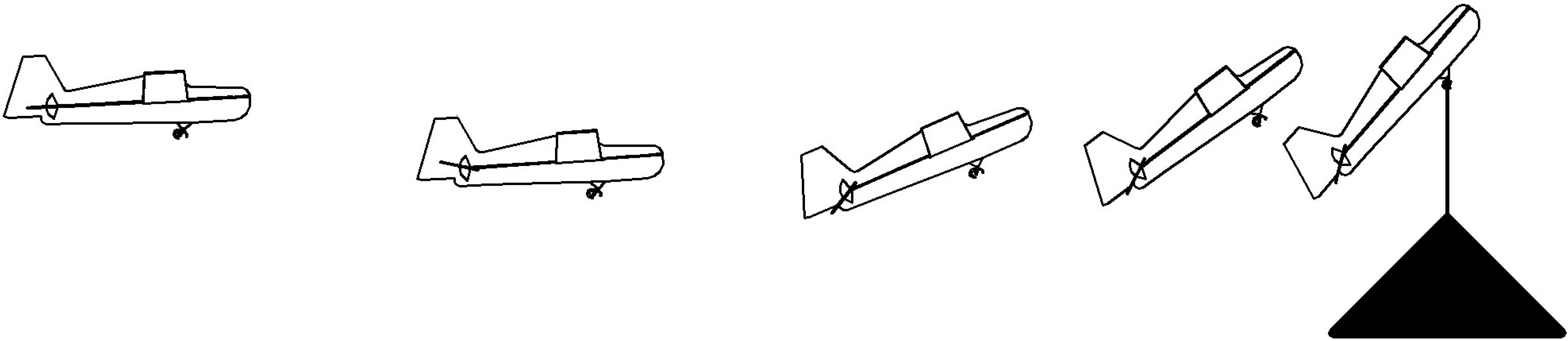
At the outset, this was a daunting task. When birds land on a perch, they pitch up and expose their wings to an "angle-of-attack" that far exceeds the typical flight envelope. Airplanes traditionally work hard to avoid this regime because it leads to aerodynamic "stall" -- a sudden loss of lift after the airflow separates from the wing. But this loss of lift is also accompanied by a significant increase in drag, and birds exploit this when they rapidly decelerate to land on a perch. Post-stall aerodynamics are a challenge for control because (1) the aerodynamics are time-varying (characterized by periodic vortex shedding) and nonlinear, (2) it is much harder to build accurate models of this flight regime, at least in a wind tunnel, and (3) stall implies a loss of attached flow on the wing and therefore on the control surfaces, so a potentially large reduction in control authority.
We picked the project initially thinking that it would be a nice example
for model-free control (like reinforcement learning -- since the models
were unknown). In the end, however, it turned out to be the project that
really taught me about the power of model-based trajectory optimization and
linear optimal control. By conducting dynamic system identification
experiments in a motion capture environment, we were able to fit both
surprisingly simple models (based on flat-plate theory) to the
dynamics
I was wrong. Over and over again, I watched time-varying linear quadratic regulators take highly nontrivial corrective actions -- for instance, dipping down early in the trajectory to gain kinetic energy or tipping up to dump energy out of the system -- in order to land on the perch at the final time. Although the quality of the linear approximation of the dynamics did degrade the farther that we got from the nominal trajectory, the validity of the controller dropped off much less quickly (even as the vector field changed, the direction that the controller needed to push did not). This was also the thinking that got me initially so interested in understanding the regions of attraction of linear control on nonlinear systems.
In the end, the experiments were very successful. We started searching for the "simplest" aircraft that we could build that would capture the essential control dynamics, reduce complexity, and still accomplish the task. We ended up building a series of flat-plate foam gliders (no propeller) with only a single actuator to control the elevator. We added dihedral to the wings to help the aircraft stay in the longitudinal plane. The simplicity of these aircraft, plus the fact that they could be understood through the lens of quite simple models makes them one of my favorite canonical underactuated systems.
The Flat-Plate Glider Model

In our experiments, we found the dynamics of our aircraft
Trajectory optimization
Trajectory stabilization


Trajectory funnels

Beyond a single trajectory
The linear controller around a nominal trajectory was surprisingly effective, but it's not enough. We'll return to this example again when we talk about "feedback motion planning", in order to discuss how to find a controller that can work for many more initial conditions -- ideally all of the initial conditions of interest for which the aircraft is capable of getting to the goal.
Pontryagin's Minimum Principle
The tools that we've been developing for numerical trajectory optimization are closely tied to theorems from (analytical) optimal control. Let us take one section to appreciate those connections.
What precisely does it mean for a trajectory, $\bx(\cdot),\bu(\cdot)$, to be locally optimal? It means that if I were to perturb that trajectory in any way (e.g. change $\bu_3$ by $\epsilon$), then I would either incur higher cost in my objective function or violate a constraint. For an unconstrained optimization, a necessary condition for local optimality is that the gradient of the objective at the solution be exactly zero. Of course the gradient can also vanish at local maxima or saddle points, but it certainly must vanish at local minima. We can generalize this argument to constrained optimization using Lagrange multipliers.
Lagrange multiplier derivation of the adjoint equations
Let us use Lagrange multipliers to derive the necessary conditions for our constrained trajectory optimization problem in discrete time \begin{align*} \min_{\bx[\cdot],\bu[\cdot]} & \ell_f(\bx[N]) + \sum_{n=0}^{N-1} \ell(\bx[n],\bu[n]),\\ \subjto \quad & \bx[n+1] = f_d(\bx[n],\bu[n]). \end{align*} Formulate the Lagrangian, \[L(\bx[\cdot],\bu[\cdot],\lambda[\cdot]) = \ell_f(\bx[N]) + \sum_{n=0}^{N-1} \ell(\bx[n],\bu[n]) + \sum_{n=0}^{N-1} \lambda^T[n] \left(f_d(\bx[n],\bu[n]) - \bx[n+1]\right), \] and set the derivatives to zero to obtain the adjoint equation method described for the shooting algorithm above: \begin{gather*} \forall n\in[0,N-1], \pd{L}{\lambda[n]} = f_d(\bx[n],\bu[n]) - \bx[n+1] = 0 \Rightarrow \bx[n+1] = f(\bx[n],\bu[n]) \\ \forall n\in[0,N-1], \pd{L}{\bx[n]} = \pd{\ell(\bx[n],\bu[n])}{\bx} + \lambda^T[n] \pd{f_d(\bx[n],\bu[n])}{\bx} - \lambda^T[n-1] = 0 \\ \quad \Rightarrow \lambda[n-1] = \pd{\ell(\bx[n],\bu[n])}{\bx}^T + \pd{f_d(\bx[n],\bu[n])}{\bx}^T \lambda[n]. \\ \pd{L}{\bx[N]} = \pd{\ell_f}{\bx}^T - \lambda^T[N-1] = 0 \Rightarrow \lambda[N-1] = \pd{\ell_f}{\bx} \\ \forall n\in[0,N-1], \pd{L}{\bu[n]} = \pd{\ell(\bx[n],\bu[n])}{\bu} + \lambda^T[n] \pd{f_d(\bx[n],\bu[n])}{\bu} = 0. \end{gather*} Therefore, if we are given an initial condition $\bx_0$ and an input trajectory $\bu[\cdot]$, we can verify that it satisfies the necessary conditions for optimality by simulating the system forward in time to solve for $\bx[\cdot]$, solving the adjoint equation backwards in time to solve for $\lambda[\cdot]$, and verifying that $\pd{L}{\bu[n]} = 0$ for all $n$. The fact that $\pd{J}{\bu} = \pd{L}{\bu}$ when $\pd{L}{\bx} = 0$ and $\pd{L}{\lambda} = 0$ follows from some basic results in the calculus of variations.
Necessary conditions for optimality in continuous time
You won't be surprised to hear that these necessary conditions have an analogue in continuous time. I'll state it here without derivation. Given the initial conditions, $\bx_0$, a continuous dynamics, $\dot\bx = f(\bx,\bu)$, and the instantaneous cost $\ell(\bx,\bu)$, for a trajectory $\bx(\cdot),\bu(\cdot)$ defined over $t\in[t_0,t_f]$ to be optimal it must satisfy the conditions that \begin{align*} \forall t\in[t_0,t_f],\quad & \dot{\bx} = f(\bx,\bu), \quad &\bx(0)=\bx_0\\ \forall t\in[t_0,t_f],\quad & -\dot\lambda = \pd{\ell}{\bx}^T + \pd{f}{\bx}^T \lambda, \quad &\lambda(T) = \pd{\ell_f}{\bx}^T \\ \forall t\in[t_0,t_f],\quad & \pd{\ell}{\bu} + \lambda^T\pd{f}{\bu} = 0.& \end{align*}
In fact the statement can be generalized even beyond this to the case where $\bu$ has constraints. The result is known as Pontryagin's minimum principle -- giving necessary conditions for a trajectory to be optimal.
Pontryagin's Minimum Principle
Adapted from
Note that the terms which are minimized in the final line of the theorem are commonly referred to as the Hamiltonian of the optimal control problem, $$H(\bx,\bu,\lambda,t) = \ell(\bx,\bu) + \lambda^T f(\bx,\bu).$$ It is distinct from, but inspired by, the Hamiltonian of classical mechanics. Remembering that $\lambda$ has an interpretation as $\pd{J}{\bx}^T$, you should also recognize it from the HJB.
Variations and Extensions
Differential Flatness
There are some very important cases where nonconvex trajectory optimization can be turned back into convex trajectory optimization based on a clever change of variables. One of the key ideas in this space is the notion of "differential flatness", which is philosophically quite close to the idea of partial feedback linearization that we discussed for acrobots and cart-pole systems. But perhaps the most famous application of differential flatness, which we will explore here, is actually for quadrotors.
One of the most important lessons from partial feedback linearization, is the idea that if you have $m$ actuators, then you basically get to control exactly $m$ quantities of your system. Differential flatness exploits this same idea (choosing $m$ outputs), but in the opposite direction. The idea is that, for some systems, if you give me a trajectory in those $m$ coordinates, it may in fact dictate what all of the states/actuators must have been doing. The fact that you can only execute a subset of possible trajectories can, in this case, make trajectory planning much easier!
Let's start with an example...
Differential flatness for the Planar Quadrotor
The planar quadrotor model described earlier has 3 degrees of freedom ($x,y,\theta$) but only two actuators (one for each propeller). My claim is that, if you give me a trajectory for just the location of the center of mass: $x(t), y(t), \forall t \in [t_0, t_f],$ then I will be able to infer what $\theta(t)$ must be over that same interval in order to be feasible. Furthermore, I can even infer $\bu(t)$. There is one technical condition required: the trajectory you give me for $x(t)$ and $y(t)$ needs to be continuously differentiable (four times).
To see this, recall the equations of motion for this system were given by: \begin{gather} m \ddot{x} = -(u_1 + u_2)\sin\theta, \label{eq:quad_x}\\ m \ddot{y} = (u_1 + u_2)\cos\theta - mg, \label{eq:quad_y}\\ I \ddot\theta = r (u_1 - u_2) \label{eq:quad_theta} \end{gather} Observe that from ($\ref{eq:quad_x}$) and ($\ref{eq:quad_y}$) we have $$\frac{-m \ddot{x}}{ m \ddot{y} + mg} = \frac{(u_1 + u_2)\sin\theta}{(u_1+u_2)\cos\theta} = \tan\theta.$$ In words, given $\ddot{x}(t)$ and $\ddot{y}(t)$, I can solve for $\theta$(t). I can differentiate this relationship (in time) twice more to obtain $\ddot\theta$. Using ($\ref{eq:quad_theta}$) with ($\ref{eq:quad_x}$) or ($\ref{eq:quad_y}$) give us two linear equations for $u_1$ and $u_2$ which are easily solved.
Now you can see why we need the original trajectories to be smooth -- the solution to $\bu(t)$ depends on $\ddot\theta(t)$ which depends on $\frac{d^4 x(t)}{dt^4}$ and $\frac{d^4 y(t)}{dt^4}$; we need those derivatives to exist along the entire trajectory.
What's more -- if we ignore input limits for a moment -- any sufficiently smooth trajectory of $x(t), y(t)$ is feasible, so if I can simply find one that avoids the obstacles, then I have designed my state trajectory. As we will see, optimizing even high-degree piecewise-polynomials is actually an easy problem (it works out to be a quadratic program), assuming the constraints are convex. In practice, this means that once you have determined whether to go left or right around the obstacles, trajectory design is easy and fast.
I've coded up a simple example of that for you here:

The example above demonstrates that the planar quadrotor system is
differentially flat in the outputs $x(t)$, $y(t)$. More generally, if we
have a dynamical system $$\dot{\bx} = f(\bx, \bu),$$ and we design some
output coordinates (essentially "task-space"): $$\bz(t) = h\left(\bx, \bu,
\frac{d\bu}{dt}, ..., \frac{d^k\bu}{dt^k}\right),$$ such that we can write
the $\bx$ and $\bu$ purely as a function of the output and it's time
derivatives, \begin{gather*} \bx (t) = \bx\left(\bz, \frac{d\bz}{dt}, ...,
\frac{d^k\bz}{dt^k}\right), \\ \bu (t) = \bu\left(\bz, \frac{d\bz}{dt}, ..,
\frac{d^k\bz}{dt^k}\right),\end{gather*} then we say that the system $f$ is
differentially flat in the outputs $\bz$
I'm not aware of any numerical recipes for showing that a system is differentially flat nor for finding potential flat outputs, but I admit I haven't worked on it nor looked for those recipes. That would be interesting! I think of differential flatness as a property that one must find for your system -- typically via a little mechanical intuition and a lot of algebra. Once found, it can be very useful.
Differential flatness for the 3D Quadrotor
Probably the most famous example of differential flatness is on the
full 3D quadrotors.
A few things to note about these examples, just so we also understand the limitations. First, the technique above is great for designing trajectories, but additional work is required to stabilizing those trajectories (we'll cover that topic in more detail later in the notes). Trajectory stabilization benefits greatly from good state estimation, and the examples above were all performed in a motion capture arena. Also, the "simple" version of the trajectory design that is fast enough to be used for flying through moving hoops is restricted to convex optimization formulations -- which means one has to hard-code apriori the decisions about whether to go left or right / up or down around each obstacle.
Iterative LQR and Differential Dynamic Programming
There is another approach to trajectory optimization (at least for
initial-value problems) that has gotten quite popular lately. Iterative
LQR (iLQR)
The motivation behind iterative LQR is quite appealing -- it
leverages the surprising structure of the Riccati equations to come up
with a second-order update to the trajectory after a single backward
pass of the Riccati equation followed by a forward simulation.
Anecdotally, the convergence is fast and robust. Numerous
applications...
One key limitation of iLQR is that it only supports unconstrained trajectory optimization -- at least via the Riccati solution. The natural extension for constrained optimization would be to replace the Riccati solution with an iterative linear model-predictive control (MPC) optimization; this would result in a quadratic program and is very close to what is happening in SQP. But a more common approach in the current robotics literature is to add any constraints into the objective function using penalty methods, especially using Augmented Lagrangian.
Differential Dynamic Programming (DDP)
Leveraging combinatorial optimization
Many of the nonconvex costs and constraints that we have been dealing with (or
avoiding!) can naturally be represented as "disjunctive" constraints (e.g. $x \in
A$ or $x \in B$). There has been an important series of work showing how
mixed-integer programming can be used, for instance, to perform trajectory
optimziation around obstacles
Recently this approach to trajectory optimization has gotten dramatically more effective using a new framework call Graphs of Convex Sets" (GCS). GCS provides a much more efficient transcription for many of the discrete+continuous trajectory optimization problems. In many cases, the convex relaxation of the mixed-integer problem is tight enough that one only needs to solve the convex relaxation (followed by a little "rounding") to solve the problem to global optimality.
Minimum-time linear optimal control
Recall our first example of the chapter was doing trajectory optimization for the double integrator. Optimizing convex objectives over a fixed horizon is naturally transcribed into convex optimization problem. But in order to solve the minimum-time problem (where the horizon is unknown), we had to solve multiple optimization problems to find the correct horizon.
This search over horizon can naturally be encoded as a mixed-integer problem, and GCS provides a natural and efficient framework for doing it. First, let's observe that the original fixed-horizon problem can naturally be described as a GCS: take the sets to be the domain of $x$ (to make these domains bounded, one can simply pick a conservative bounding box). Our graph will simply be a serial chain with one copy of this set for each timestep, and edge constraints that enforce the dynamics: $$\bx[n+1] - \bA \bx[n] \in \bB {\bf U},\qquad {\bf U} = \left\{ \begin{bmatrix}u\end{bmatrix} \, | \, u \in [-1, 1] \right\}.$$ Awesomely, once we implement all of the code optimizations that we are currently working on for Drake's GCS implementation, formulating the problem in this way will give you back exactly the same linear program that we solved above.
Now we can make the time duration optional by defining edges, with constraints, from each timestep directly to the goal:

Note that for this example, the GCS convex relaxation is not tight (yet; I
still have some ideas), but the convex_relaxation = False version
solves beautifully, if you have an MIP solver available.
The minimum-time double integrator problem is too simple to warrant the use of GCS. Afterall, the line search we recommended above can work efficiently enough. But this is a nice simple illustration of how one might formulate trajectory optimization as a GCS, and it will scale to much more complicated formulations.
MPC for piecewise-affine systems (PWAMPC)
Motion planning around obstacles
Let's consider the simple problem of planning a path (even without any dynamics) for a point robot moving around an obstacle. This is our canonical example of a non-convex constraint that we might encounter in our trajectory optimization formulations.
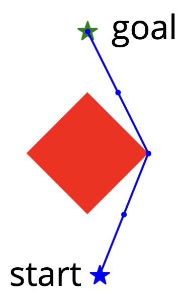
In the notebook below, I've implemented a handful of different ways to transcribe this into an optimization problem.
Minimum-snap trajectories for quadrotors flying around obstacles
More recently,
Try it out for yourself:

You can check out the trajectories in the meshcat animation.
Explicit model-predictive control
We do actually understand what the optimal policy of the
inequality-constrained LQR problem looks like, thanks to work on
"explicit MPC"
Exercises
Direct Shooting vs Direct Transcription
In this coding exercise we explore in detail the computational advantages of direct transcription over direct shooting methods. The exercise can be completed entirely in . To simplify the analysis, we will apply these two methods to a finite-horizon LQR problem. You are asked to complete four pieces of code:
- Use the given implementation of direct shooting to analyze the numerical conditioning of this approach.
- Complete the given implementation of the direct transcription method.
- Verify that the cost to go from direct trascription approaches the LQR cost to go as the time horizon grows.
- Analyze the numerical conditioning of direct transcription.
- Implement the dynamic programming recursion (a.k.a. "Riccati recursion") to efficiently solve the linear algebra underlying the direct transcription method.
Orbital Transfer via Trajectory Optimization
For this exercise you will work exclusively in . You are asked to find, via nonlinear trajectory optimization, a path that efficiently transfers a rocket from the Earth to Mars, while avoiding a cloud of asteroids. The skeleton of the optimization problem is already there, but several important pieces are missing. More details are in the notebook, but you will need to:
- Enforce the maximum thrust constraints.
- Enforce the maximum velocity constraints.
- Ensure that the rocket does not collide with any of the asteroids.
- Add an objective function to minimize fuel consumption.
Iterative Linear Quadratic Regulator: Theory
Please read sections 1 and 2 of this paper
- What optimization problem is iLQR solving? What is the output of the algorithm?
- Explain what the backward pass does and what purpose it serves.
- Explain what the forward pass does and what purpose it serves.
- Explain how the two interact with each other in an iterative manner. Do you expect the algorithm to converge? Why?
- Explain the difference between DDP and iLQR.
- Suppose the system dynamics aren't smooth (i.e., not continuously differentiable), but are still available in closed form. Can you still apply the algorithm? Would the backward pass still work? What about the forward pass?
Iterative Linear Quadratic Regulator: Implementation
The exercise is self-contained in . In this exercise you will derive and implement the iterative Linear Quadratic Regulator (iLQR). You will evaluate it's functionality by planning trajectories for an autonomous vehicle. You will need to:
- Define an integrator for continuous dynamics.
- Compute a trajectory given an initial state and a control trajectory.
- Sum up the total cost of that trajectory.
- Derive the coefficients of the quadratic Q-function.
- Optimize for the optimal control law.
- Derive the update of the value function backwards in time.
- Implement the forward pass of iLQR.
- Implement the backward pass of iLQR.
Differential Flatness
Consider a planar rigid body of mass $m$ and moment of inertia $I$ moving under the influence of gravity and forces $F_1$ and $F_2$ acting at point $P$ of the body (shown in image). The state of the body at any time is defined by $\mathbf{x} = (x, y, \theta)$ where $x$ and $y$ are the COM positions and $\theta$ is the orientation of the body, respectively. The equations of motion are given by: \begin{align*} m\ddot{x} &= F_1 \cos \theta + F_2 \sin \theta \\ m\ddot{y} &= F_1 \sin \theta - F_2 \cos \theta - mg \\ I\ddot{\theta} &= rF_1 \end{align*}
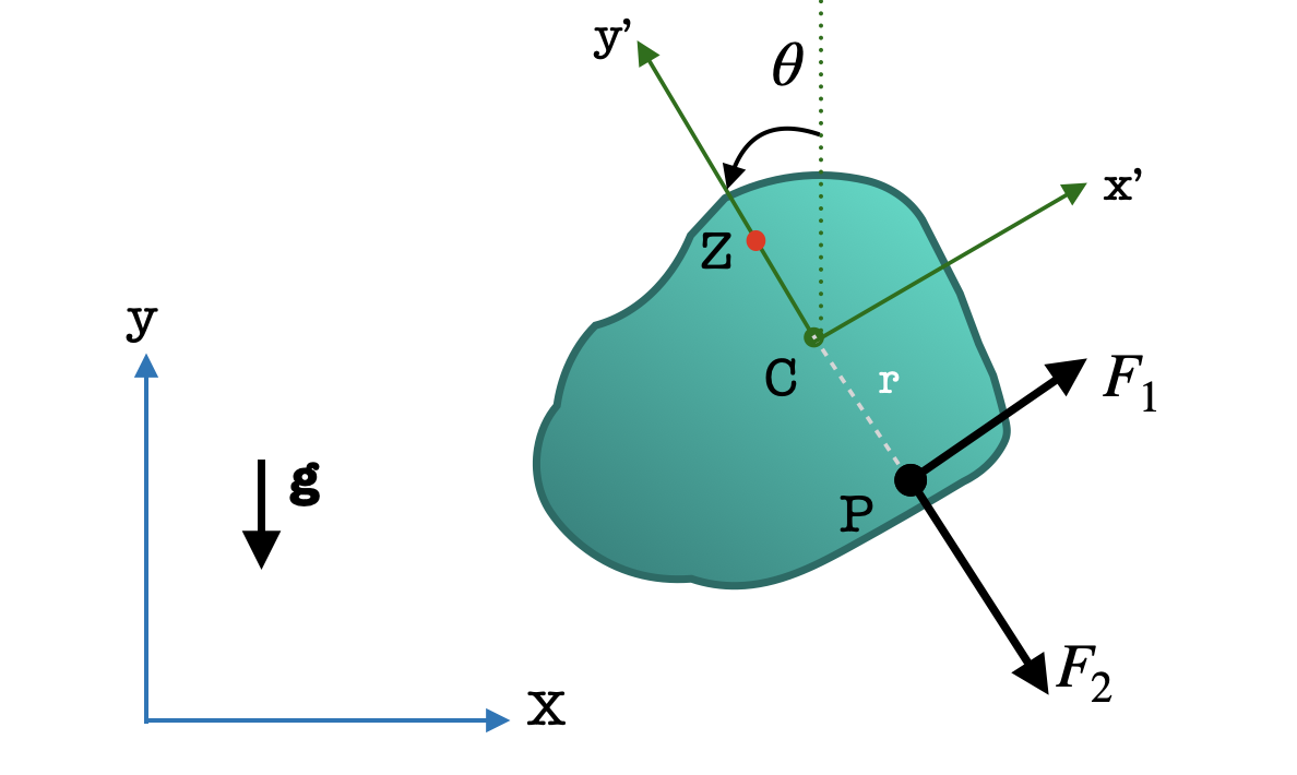
- Show that the system is differentially flat in the output $Z$, the center of oscillation, given by $\mathbf{z} = (z_1, z_2)$
\begin{equation*}
z_1 = x - \frac{I}{mr} \sin \theta \quad \quad
z_2 = y + \frac{I}{mr} \cos \theta
\end{equation*}
In other words, you must show that given a sufficiently differentiable trajectory $\mathbf{z}(t)$,
you can uniquely determine the trajectory $\mathbf{x}(t)$ (upto an ambiguity of $\pi$ in $\theta$).
Hint: Show that $\theta$ is uniquely determined by some high order derivatives of $z_1$ and $z_2$. Then show that $\ddot x_1$ and $\ddot x_2$ are uniquely determined by some high order derivatives $z_1$ and $z_2$.
Hint: Section 10.8.1 and Example 10.3 are a good reference. Substitute $\ddot{z}_1$, $\ddot{z}_2$ into the expressions for $\ddot{x}$ and $\ddot{y}$. -
Suppose we can control the magnitude of forces $F_1$ and $F_2$ that act at point $P$, and that there are no constraints on $F_1$ and $F_2$.
We wish to find a trajectory (control and state) such that the body passes through certain waypoints $(x_k,y_k,\theta_k)$.
- Explain how we can use differentially flat coordinates to produce such a trajectory.
- Explain the difference between trajectory planning formulations in the original coordinates $\mathbf x$ and the differentially flat coordinates $\mathbf z$. Are they convex? Which one is easier to solve and why?
- Suppose the magnitudes of forces $F_1$ and $F_2$ are constrained to be less than $F_{max}$. How will this affect the trajectory optimization in the differentiably flat coordinates? In particular, will the resulting optimization be convex?