Simple Models of Walking and Running
Practical legged locomotion is one of the fundamental problems in robotics; we've seen amazing progress over the last few years, but there are still some major unsolved problems. Much of the recent progress is due to improvements in hardware -- a legged robot must carry all of its sensors, actuators and power and traditionally this meant underpowered motors that act as far-from-ideal force/torque sources -- Boston Dynamics and other companies have made incredible progress here. The control systems implemented on these systems, though, are still more heuristic than you might think. They also require dramatically higher bandwidth and lower latency than the human motor control system and still perform worse in challenging environments.
The control of walking robots is definitely underactuated: assuming we
cannot pull on the ground (and barring any aerodynamic effects!), then no
matter how powerful my actuators are, there is nothing that we can do to
accelerate the center of mass of the robot towards the ground faster than
gravity. But beyond the underactuated systems we have studied so far, the
control of walking robots faces an additional complexity: controlling
through contact. The fact that we can get non-zero contact forces if and
only if two bodies are in contact introduces a fundamentally
discrete/combinatorial element into the problem†
Contact is essential for many aspects of robotics (manipulation is my other favorite example); it's sad to see so many robots going through life avoiding contact at any cost. Controlling contact means that your robot is capable of performing physical work on the environment; isn't that the point of robotics, afterall?
I like to start our discussion of contact with walking robots for a few important reasons. As you'll see in this chapter, there are a number of elegant "simple models" of walking that capture much of the essence of the problem with minimal complexity. But there is another, more subtle, reason: I want to continue to use the language of stability. At this point we've seen both finite-horizon and infinite-horizon problem formulations -- when we can say something about the behavior of a system in the limit as time goes to infinity, it's almost always cleaner than a finite-time analysis (because time drops away). Walking provides a very clean way to use the language of stability in studying behavior of systems that are sometimes in contact but sometimes out of contact in the limiting case; we just need to extend our notions from stability of a fixed point to the stability of a (periodic) cycle.
Limit Cycles
A limit cycle is an periodic orbit that is a limit set of the dynamical system; they can be stable (the limit set of neighboring trajectories as time goes to infinity) or unstable (the limit set of neighboring trajectories as time goes to negative infinity). One of the simplest models of limit cycle behavior is the Van der Pol oscillator. Let's examine that first...
Van der Pol Oscillator
The Van der Pol oscillator is described by a second-order differential equation in one variable: $$\ddot{q} + \mu (q^2 - 1)\dot{q} + q = 0, \quad \mu>0$$ One can think of this system as almost a simple spring-mass-damper system, except that it has nonlinear damping. In particular, the velocity term dissipates energy when $|q|>1$, and adds energy when $|q|<1$. Therefore, it is not terribly surprising to see that the system settles into a stable oscillation from almost any initial conditions (the exception is the state $q=0,\dot{q}=0$). This can be seen nicely in the phase portrait below.

|

|
However, if we examine system trajectories in the time domain (see the right panel of the figure above), then we can see that our traditional notion for stability of a trajectory, $\lim_{t\rightarrow \infty} |\bx(t) - \bx^*(t)| = 0$, is not satisfied here for any $\bx^*(t)$. Although the phase portrait clearly reveals that all trajectories converge to the same orbit, the time domain plot reveals that these trajectories do not necessarily synchronize in time.
This example shows that stability of a trajectory (in time) is not the definition we want. Instead we will define the stability of an orbit, $\bx^*(t)$, using \[ \min_\tau || \bx(t) - \bx^*(\tau) ||.\] Here the quantity of interest is the distance between our trajectory and the closest point on the orbit. Depending on exactly how this distance evolves with time, we can define orbital stability: for every small $\epsilon>0$, we can find a $\delta>0$ such that $\min_\tau||\bx(t_0) - \bx^*(\tau)|| < \delta$ implies $\forall t, \min_\tau ||\bx(t) - \bx^*(\tau)|| < \epsilon$). The definitions for asymptotic orbital stability, exponential orbital stability, finite-time orbital stability follow naturally, as does the definition of an unstable orbit. In the case of limit cycles, this $\bx^*(t)$ is a periodic solution with $\bx^*(t+t_{period}) = \bx^*(t)$.
As we begin to extend our notions of stability, allow me to make a few
quick connections to the discussion of stability in the chapter on Lyapunov analysis. It's interesting to
know that if we can find an invariant
set in state space which does not contain any fixed points, then this
set must contain a closed orbit (this is the Poincaré-Bendixson
Theorem)
Poincaré Maps
The first tool one should know for analyzing the stability of a limit cycle, and one that will serve us quite well for the examples in this chapter, is the method of Poincaré. Let's consider a dynamical system, $\dot{\bx} = {\bf f}(\bx),$ with $\bx \in \Re^n.$ Define an $n-1$ dimensional surface of section, $S$. We will also require that $S$ is transverse to the flow (i.e., all trajectories starting on $S$ flow through $S$, not parallel to it). The Poincaré map (or return map) is a mapping from $S$ to itself: $$\bx_p[n+1] = {\bf P}(\bx_p[n]),$$ where $\bx_p[n]$ is the state of the system at the $n$th crossing of the surface of section. Note that we will use the notation $\bx_p$ to distinguish the state of the discrete-time system from the continuous-time system; they are related by $\bx_p[n] = \bx(t_c[n])$, where $t_c[n]$ is the time of the $n$th crossing of $S$.
For our purposes in this chapter, it will be useful for us to allow the Poincaré maps to also include fixed points of the original continuous-time system, and to define the return time to be zero. These points do not satisfy the transversality condition, and require some care numerically, but they do not compromise our analysis.
Return map for the Van der Pol Oscillator
Since the state space of this system is two-dimensional, a return map for the system must have dimension one. For instance, we can take $S$ to be the line segment where $q = 0$, $\dot{q} \ge 0$. It is easy to see that all trajectories that start on S are transverse to it.
One dimensional maps, like one dimensional flows, are amenable to graphical analysis.
 |  |
If we can demonstrate that ${\bf P}(\bx_p)$ exists for all $\bx_p \in S$, (all trajectories that leave $S$ eventually return to $S$), then something remarkable happens: we can reduce the stability analysis for a limit cycle in the original coordinates into the stability analysis of a fixed point on the discrete map. If $\bx^*_p$ is a stable (or unstable) fixed point of the map ${\bf P}$, then there exists a unique periodic orbit $\bx^*(t)$ which passes through $\bx^*_p$ that is a (stable, or unstable) limit cycle. If we are able to upper-bound the time it takes for trajectories leaving $S$ to return, then it is also possible to infer asympotitic orbital or even exponential orbital stability.
In practice it is often difficult or impossible to find ${\bf P}$ analytically, but it can be sampled quite reasonably numerically. Once a fixed point of ${\bf P}$ is obtained (by finding a solution to $\bx^*_p = {\bf P}(\bx^*_p)$), we can infer local limit cycle stability with an eigenvalue analysis. If this eigen-analysis is performed in the original coordinates (as opposed to the $n-1$ dimensional coordinates of $S$), then there will always be a at least one zero eigenvalue - corresponding to perturbations along the limit cycle which do not change the state of first return. The limit cycle is considered locally exponentially stable if all remaining eigenvalues, $\lambda_i$, have magnitude less than one, $|\lambda_i|<1$.
It is sometimes possible to infer more global stability properties of
the return map by examining ${\bf P}$. We will study computational
methods in the later chapter.
A particularly graphical method for understanding the dynamics of a one-dimensional iterated map is the "staircase method": Sketch the Poincaré map -- a plot of $x_p[n]$ vs $x_p[n+1]$ -- and also the line of slope one. In order to "iterate" the map, take an initial condition on the plot as a point $\left( x_p[k], x_p[k] \right)$, and move vertically on the plot to the point $\left( x_p[k], x_p[k+1] = f(x_p[k]) \right)$. Now move horizontally to the next point $\left( x_p[k+1], x_p[k+1] \right)$ and repeat.

We can quickly recognize the fixed points as the points where the return map crosses this line. We can infer local exponential stability if the absolute value of the slope of return map at the fixed point is less than one ($|\lambda| < 1$). The figure above illustrates the stability of the Van der Pol limit cycle; it also illustrates the (one-sided) instability of the fixed point at the origin. Understanding the regions of attraction of fixed points on an iterated map (or any discrete-time system) graphically requires a little more care, though, than the continuous-time flows we examined before. The discrete maps can jump a finite distance on each step, and will in fact oscillate back and forth from either side of the fixed point when $\lambda < 0.$
Simple Models of Walking
Much of the fundamental work in the dynamics of legged robots was done originally in the context of studying passive-dynamic walkers (often just "passive walker"). We've already seen my favorite example of a passive walker, in the first chapter, but here it is again:
This amazing robot has no motors and no controllers... it walks down a tiny ramp and is powered entirely by gravity. We can build up our understanding of this robot in a series of steps. As we will see, what is remarkable is that even though the system is passive, the periodic gait you see in the video is actually a stable limit cycle!
Well before the first passive walkers, one of the earliest models of
walking was proposed by McMahon
The Rimless Wheel

Perhaps the simplest possible model of a legged robot, introduced as
the conceptual framework for passive-dynamic walking by
McGeer
- Collisions with ground are inelastic and impulsive (only angular momentum is conserved around the point of collision).
- The stance foot acts as a pin joint and does not slip.
- The transfer of support at the time of contact is instantaneous (no double support phase).
- $0 \le \gamma < \frac{\pi}{2}$, $0 < \alpha < \frac{\pi}{2}$, $l > 0$.
Note that the coordinate system used here is slightly different than for the simple pendulum ($\theta=0$ is at the top, and the sign of $\theta$ has changed).
The most comprehensive analysis of the rimless wheel was done by
Stance Dynamics
The dynamics of the system when one leg is on the ground are given by $$\ddot\theta = \frac{g}{l}\sin(\theta).$$ If we assume that the system is started in a configuration directly after a transfer of support ($\theta(0^+) = \gamma-\alpha$), then forward walking occurs when the system has an initial velocity, $\dot\theta(0^+) > \omega_1,$ where $$\omega_1 = \sqrt{ 2 \frac{g}{l} \left[ 1 - \cos \left (\gamma-\alpha \right) \right]}.$$ $\omega_1$ is the threshold at which the system has enough kinetic energy to vault the mass over the stance leg and take a step. This threshold is zero for $\gamma = \alpha$ and does not exist for $\gamma > \alpha$ (because when $\gamma > \alpha$ the mass is always ahead of the stance foot, and the standing fixed point disappears). The next foot touches down when $\theta(t) = \gamma+\alpha$, at which point the conversion of potential energy into kinetic energy yields the velocity $$\dot\theta(t^-) = \sqrt{\dot\theta^2(0^+) + 4\frac{g}{l} \sin\alpha \sin\gamma }.$$ $t^-$ denotes the time immediately before the collision.
Foot Collision

The angular momentum around the point of collision at time $t$ just before the next foot collides with the ground is $$L(t^-) = -ml^2\dot\theta(t^-) \cos(2\alpha).$$ The angular momentum at the same point immediately after the collision is $$L(t^+) = -ml^2\dot\theta(t^+).$$ Assuming angular momentum is conserved, this collision causes an instantaneous loss of velocity: $$\dot\theta(t^+) = \dot\theta(t^-) \cos(2\alpha).$$
Forward simulation
Given the stance dynamics, the collision detection logic ($\theta = \gamma \pm \alpha$), and the collision update, we can numerically simulate this simple model. Doing so reveals something remarkable... the wheel starts rolling, but then one of two things happens: it either runs out of energy and stands still, or it quickly falls into a stable periodic solution. Convergence to this stable periodic solution appears to happen from a huge range of initial conditions. Try it yourself.
Numerical simulation of the rimless wheel
I've setup the notebook to make it easy for you to try a handful of interesting initial conditions. And even made an interactive widget for you to watch the simulation phase portrait as you change those initial conditions. Give it a try!
The rimless wheel model actually uses a number of
the more nuanced features of

One of the fantastic things about the rimless wheel is that the dynamics are exactly the undamped simple pendulum that we've thought so much about. So you will recognize the phase portraits of the system -- they are centered around the unstable fixed point of the simple pendulum.
Poincaré Map
We can now derive the angular velocity at the beginning of each stance phase as a function of the angular velocity of the previous stance phase. First, we will handle the case where $\gamma \le \alpha$ and $\dot\theta_n^+ > \omega_1$. The "step-to-step return map", factoring losses from a single collision, the resulting map is: $$\dot\theta^{+}_{n+1} = \cos(2\alpha) \sqrt{ ({\dot\theta_n}^{+})^{2} + 4\frac{g}{l}\sin\alpha \sin\gamma}.$$ where the $\dot{\theta}^{+}$ indicates the velocity just after the energy loss at impact has occurred.
Using the same analysis for the remaining cases, we can complete the return map. The threshold for taking a step in the opposite direction is $$\omega_2 = - \sqrt{2 \frac{g}{l} [1 - \cos(\alpha + \gamma)]}.$$ For $\omega_2 < \dot\theta_n^{+} < \omega_1,$ we have $$\dot\theta_{n+1}^{+} = -\dot\theta_n^{+} \cos(2\alpha).$$ Finally, for $\dot\theta_n^{+} < \omega_2$, we have $$\dot\theta_{n+1}^{+} = - \cos(2\alpha)\sqrt{(\dot\theta_n^{+})^2 - 4 \frac{g}{l} \sin\alpha \sin\gamma}.$$ Altogether, we have (for $\gamma \le \alpha$) $$\dot\theta_{n+1}^{+} = \begin{cases} \cos(2\alpha) \sqrt{(\dot\theta_n^{+})^2 + 4 \frac{g}{l} \sin\alpha \sin\gamma}, & \text{ } \omega_1 < \dot\theta_n^{+} \\ -\dot\theta_n^{+} \cos(2\alpha), & \text{ } \omega_2 < \dot\theta_n^{+} < \omega_1 \\ -\cos(2\alpha) \sqrt{(\dot\theta_n^{+})^2 - 4\frac{g}{l} \sin\alpha \sin\gamma}, & \dot\theta_n^{+} < w_2 \end{cases}.$$
Notice that the return map is undefined for $\dot\theta_n = \{ \omega_1, \omega_2 \}$, because from these configurations, the wheel will end up in the (unstable) equilibrium point where $\theta = 0$ and $\dot\theta = 0$, and will therefore never return to the map.
This return map blends smoothly into the case where $\gamma > \alpha$. In this regime, $$\dot\theta_{n+1}^{+} = \begin{cases} \cos(2\alpha) \sqrt{(\dot\theta_n^{+})^2 + 4 \frac{g}{l} \sin\alpha \sin\gamma}, & \text{ } 0 \le \dot\theta_n^{+} \\ -\dot\theta_n^{+} \cos(2\alpha), & \text{ } \omega_2 < \dot\theta_n^{+} < 0 \\ -\cos(2\alpha) \sqrt{(\dot\theta_n^{+})^2 - 4\frac{g}{l} \sin\alpha \sin\gamma}, & \dot\theta_n^{+} \le w_2 \end{cases}.$$ Notice that the formerly undefined points at $\{\omega_1,\omega_2\}$ are now well-defined transitions with $\omega_1 = 0$, because it is kinematically impossible to have the wheel statically balancing on a single leg.
Fixed Points and Stability
For a fixed point, we require that $\dot\theta_{n+1}^{+} = \dot\theta_n^{+} = \omega^*$. Our system has two possible fixed points, depending on the parameters: $$ \omega_{stand}^* = 0,~~~ \omega_{roll}^* = \cot(2 \alpha) \sqrt{4 \frac{g}{l} \sin\alpha\sin\gamma}.$$ The limit cycle plotted above illustrates a state-space trajectory in the vicinity of the rolling fixed point. $\omega_{stand}^*$ is a fixed point whenever $\gamma < \alpha$. $\omega_{roll}^*$ is a fixed point whenever $\omega_{roll}^* > \omega_1$. It is interesting to view these bifurcations in terms of $\gamma$. For small $\gamma$, $\omega_{stand}$ is the only fixed point, because energy lost from collisions with the ground is not compensated for by gravity. As we increase $\gamma$, we obtain a stable rolling solution, where the collisions with the ground exactly balance the conversion of gravitational potential to kinetic energy. As we increase $\gamma$ further to $\gamma > \alpha$, it becomes impossible for the center of mass of the wheel to be inside the support polygon, making standing an unstable configuration.

Stability of standing still
I opened this chapter with the idea that the natural notion of stability for a walking system is periodic stability, and I'll stand by it. But we can also examine the stability of a fixed-point (of the original coordinates; no Poincaré this time) for a system that has contact mechanics. For a legged robot, a fixed point means standing still. This can actually be a little subtle in our hybrid models: in the rimless wheel, standing still is the limiting case where we have infinitely frequent collisions. [Details coming soon.]
The Compass Gait
The rimless wheel models only the dynamics of the stance leg, and simply assumes that there will always be a swing leg in position at the time of collision. To remove this assumption, we take away all but two of the spokes, and place a pin joint at the hip. To model the dynamics of swing, we add point masses to each of the legs. I've derived the equations of motion for the system assuming that we have a torque actuator at the hip - resulting in swing dynamics equivalent to an Acrobot (although in a different coordinate frame) - but let's examine the passive dynamics of the system first ($\bu = 0$).

In addition to the modeling assumptions used for the rimless wheel, we
also assume that the swing leg retracts in order to clear the ground
without disturbing the position of the mass of that leg. This model, known
as the compass gait, is well studied in the literature using numerical
methods
The state of this robot can be described by 4 variables: $\theta_{st},\theta_{sw},\dot\theta_{st}$, and $\dot\theta_{sw}$. The abbreviation $st$ is shorthand for the stance leg and $sw$ for the swing leg. Using $\bq = [ \theta_{st}, \theta_{sw} ]^T$ and $\bu = \tau$, we can write the dynamics as $$\bM(\bq)\ddot\bq + \bC(\bq,\dot\bq)\dot\bq = \btau_g(q) + \bB\bu,$$ with \begin{gather*} \bM = \begin{bmatrix} (m_h+m)l^2 + ma^2 & -mlb\cos(\theta_{st}-\theta_{sw}) \\ -mlb\cos(\theta_{st}-\theta_{sw}) & mb^2 \end{bmatrix}\\ \bC = \begin{bmatrix} 0 & -mlb\sin(\theta_{st}-\theta_{sw})\dot\theta_{sw} \\ mlb\sin(\theta_{st}-\theta_{sw})\dot\theta_{st} & 0 \end{bmatrix} \\ \btau_g(q) = \begin{bmatrix} (m_hl + ma + ml)g\sin(\theta_{st}) \\ -mbg\sin(\theta_{sw}) \end{bmatrix},\\ \bB = \begin{bmatrix} -1 \\ 1 \end{bmatrix} \end{gather*} and $l=a+b$.
The foot collision is an instantaneous change of velocity caused by a impulsive force at the foot that brings the foot to rest. The update to the velocities can be calculated using the derivation for impulsive collisions derived in the appendix. To use it, we proceed with the following steps:
- Add a "floating base" to the system by adding a free (x,y) joint at the pre-impact stance toe, $\bq_{fb} = [x,y,\theta_{st},\theta_{sw}]^T.$
- Calculate the mass matrix for this new system, call it $\bM_{fb}$.
- Write the position of the (pre-impact) swing toe as a function $\bphi(\bq_{fb})$. Define the Jacobian of this function: $\bJ = \frac{\partial \bphi}{\partial \bq_{fb}}.$
- The post-impact velocity that ensures that $\dot\bphi = 0$ after the collision is given by $$\dot\bq^+ = \left[ \bI - \bM_{fb}^{-1}\bJ^T[\bJ\bM_{fb}^{-1}\bJ^T]^{-1}\bJ\right] \dot\bq^-,$$ noting that $\dot{x}^- = \dot{y}^- = 0$, and that you need only read out the last two elements of $\dot{\bq}^+$. The velocity of the post-impact stance foot will be zero by definition, and the new velocity of the pre-impact stance foot can be completely determined from the minimal coordinates.
- Switch the stance and swing leg positions and velocities.
Numerical simulation of the compass gait
You can simulate the passive compass gait using:
Try playing with the initial conditions. You'll find this system is much more sensitive to initial conditions than the rimless wheel. It actually took some work to find the initial conditions that make it walk stably.
Numerical integration of these equations reveals a stable limit cycle,
plotted below. Notice that when the left leg is in stance (top part of
the plot), the trajectory quite resembles the familiar pendulum dynamics
of the rimless wheel. But this time, when the leg impacts, it takes a
long arc around as the swing leg before returning to stance. The impacts
are also clearly visible as discontinuous changes (decreases) in velocity.
The dependence of this limit cycle on the system parameters has been
studied extensively in

The basin of attraction of the stable limit cycle is a narrow band of states surrounding the steady state trajectory. Although the simplicity of this model makes it attractive for conceptual explorations, this lack of stability makes it difficult to implement on a physical device.
The Kneed Walker
To achieve a more anthropomorphic gait, as well as to acquire better
foot clearance and ability to walk on rough terrain, we want to model a
walker that includes a knee

At the beginning of each step, the system is modeled as a three-link
pendulum, like the ballistic
walker
After this collision, the knee is locked and we switch to the compass gait model with a different mass distribution. In other words, the system becomes a two-link pendulum. Again, the heel-strike is modeled as an inelastic collision. After the collision, the legs switch instantaneously. After heel-strike then, we switch back to the ballistic walker's three-link pendulum dynamics. This describes a full step cycle of the kneed walker, which is shown above.

By switching between the dynamics of the continuous three-link and two-link pendulums with the two discrete collision events, we characterize a full point-feed kneed walker walking cycle. After finding appropriate parameters for masses and link lengths, a stable gait is found. As with the compass gait's limit cycle, there is a swing phase (top) and a stance phase (bottom). In addition to the two heel-strikes, there are two more instantaneous velocity changes from the knee-strikes as marked in the figure. This limit cycle is traversed clockwise.

Curved feet
The region of attraction of the kneed-walking limit cycle can be improved considerably by the addition of curved feet...
In
And beyond...
The world has seen all sorts of great variations on the passive-dynamic walker theme. Almost certainly the most impressive are the creations of Dutch artist Theo Jansen -- he likes to say that he is creating "new forms of life" which he calls the Strandbeest. There are many variations of these amazing machines -- including his beach walkers which are powered only by the wind (I've actually been able to visit Theo's workshop once; it is very windy there).
These results are very real. Robin Deits (an exceptionally talented
student who felt particularly inspired once on a long weekend) once
reproduced one of Theo's earliest creations in
Simple Models of Running
Just like walking, our understanding of the dynamics and control of running has evolved by a nice interplay between the field of biomechanics and the field of robotics. But in running, I think it's fair to say that the roboticists got off the starting blocks first. And I think it's fair to say that it started with a series of hopping machines built by Marc Raibert and the Leg Laboratory (which was first at CMU, but moved to MIT) in the early 1980's. At a time where many roboticsts were building relatively clumsy walking robots that moved very slowly (when they managed to stay up!), the Leg Laboratory produced a series of hopping machines that threw themselves through the air with considerable kinetic energy and considerable flair.
To this day, I'm still a bit surprised that impressive running robots (assuming you accept hopping as the first form of running) appeared before the impressive walking robots. I would have thought that running would be a more difficult control and engineering task than walking. But these hopping machines turned out to be an incredibly clever way to build something simple and very dynamic.
Shortly after Marc Raibert built his machines, Dan Koditschek and Martin
Buehler started analyzing them with simpler models
The Spring-Loaded Inverted Pendulum (SLIP)
The model is a point mass, $m$, on top of a massless, springy leg with rest length of $l_0$, and spring constant $k$. The configuration of the system is given by the $x,z$ position of the center of mass, and the length, $l$, and angle $\theta$ of the leg. The dynamics are modeled piecewise - with one dynamics governing the flight phase, and another governing the stance phase.

In SLIP, we actually use different state variables for each phase of the dynamics. During the flight phase, we use the state variables: $\bx = [x,z,\dot{x},\dot{z}]^T.$ The flight dynamics are simply $$\dot{\bx} = \begin{bmatrix} \dot{x} \\ \dot{z} \\ 0 \\ - g \end{bmatrix}.$$ Since the leg is massless, we assume that the leg can be controlled to any position instantaneously, so it's reasonable to take the leg angle as the control input $\theta = u$.
During the "stance phase", we write the dynamics in polar coordinates, with the foot anchored at the origin. Using the state variables: $\bx = [r, \theta, \dot{r}, \dot\theta]^T,$ the location of the mass is given by $$\bx_m = \begin{bmatrix} - r \sin\theta \\ r \cos\theta \end{bmatrix}.$$ The total energy is given by the kinetic energy (of the mass) and the potential energy from gravity and from the leg spring: $$T = \frac{m}{2} (\dot{r}^2 + r^2 \dot\theta^2 ), \quad U = mgr\cos\theta + \frac{k}{2}(l_0 - r)^2.$$ Plugging these into Lagrange yields the stance dynamics: \begin{gather*} m \ddot{r} - m r \dot\theta^2 + m g \cos\theta - k (l_0 - r) = 0, \\ m r^2 \ddot{\theta} + 2mr\dot{r}\dot\theta - mgr \sin\theta = 0.\end{gather*} We assume that the stance phase is entirely ballistic; there are no control inputs during this phase.
Unlike the rimless wheel model, the idealization of a spring leg with a massless toe means that no energy is lost during the collision with the ground. The collision event causes a transition to a different state space, and to a different dynamics model, but no instantaneous change in velocity. The transition from flight to stance happens when $z - l_0\cos\theta \le 0.$ The transition from stance to flight happens when the stance leg reaches its rest length: $r \ge l_0$.
Simulation of the SLIP model
You can simulate the spring-loaded inverted pendulum using:
Take a moment to read the code that defines the
SpringLoadedInvertedPendulum system. You can see that we
carefully register the hybrid guards (witness functions) and reset
maps, which tells the numerical integrator to use zero-crossing event
detection to isolate precisely the time of the event and to apply the
reset update at this event. It is quite elegant, and we've gone to
some length to make sure that the numerical integration routines in
We used the same witness functions and resets to simulate the walking models, but those were implemented in C++. This is a purely Python implementation, making it a bit easier to see those details.
Analysis on the apex-to-apex map
The rimless wheel had only two state variables ($\theta$, and $\dot\theta$), and since the surface of section drops one variable, we ended up with a one-dimensional Poincaré map. We have a lot more state variables here. Is there any hope for graphical analysis?
For this system, one can still make progress if we define the Poincaré section to be at the apex of the hop (when $\dot{z}=0$), and analyze the dynamics from apex to apex. We will ignore the absolute horizontal position, $x$, and the leg angle, $\theta$, as they are irrelevant to the flight dynamics. This still leaves us with two state variables at the apex: the horizontal velocity, $\dot{x},$ and the hopping height, $z$.
Importantly, at the apex, these two variables are linked -- when you
know one, you know the other. This is because no energy is ever added
or removed from the system. If you know the (constant) total energy in
the system, and you know the height at the apex, then you know the
horizontal velocity (up to a sign): $$E_{apex}(z, \dot{x}) =
\frac{1}{2}m \dot{x}^2 + mgz = E_0.$$ To make our analysis less
dependent on our specific choice of parameters, we typically report any
analysis using a dimensionless total energy, $\tilde{E} = \frac{E}{m g
l_0},$ and a dimensionless spring constant, $\tilde{k} = \frac{k
l_0}{mg}$
Putting all of these together, we can numerically evaluate the apex-to-apex return map given a known total energy of the system as a one-dimensional Poincaré map.
Numerical SLIP apex-to-apex map
Numerically integrating the equations of motion from apex-to-apex, using zero-crossing event detection, can give us the apex-to-apex map.

Using our graphical staircase analysis (for discrete-time systems), we can see that there are two fixed points of this map: one "stable" fixed point around 0.87 meters, and one unstable fixed point around 0.92 meters.
As always, you should run this code yourself to make sure you understand:
I'd also recommend running the simulation using initial conditions at various points on this plot. You should ask: why does the plot cut off so abruptly just below the stable fixed point? Well the apex-to-apex map becomes undefined if the apex is smaller that $l_0\cos\theta$ (the height at touchdown). Furthemore, when $z$ is too large (relative to $\tilde{E}$), then the system will not have enough horizontal energy to transition through the stance phase and continue forward motion: the center of mass will compress the spring and then fall backwards in the direction from which it came.
The system's conservation of total energy is quite convenient for our return map analysis, but it should give you pause. The rimless wheel actually relied on the dissipation due to collisions with the ground to acquire its stability. Is there any chance for a system that is energy conserving to be stable? The apex-to-apex return maps visualized above reveal "stable" fixed-points, but you must understand that the projection from $(z,\dot{x})$ to just $z$ is using the assumption that the energy is conserved. As a result, our analysis on the one-dimensional Poincaré map can only make a statement about partial stability (i.s.L., asymptotic, or exponential); our analysis does not say anything about stability against disturbances that change the total energy of the system.
Despite this limitation, it is quite interesting that such a simple
system converges to particular hopping heights from various initial
conditions. The observation that these "piecewise-Hamiltonian" systems
(Hamiltonian because they conserve total energy) can exhibit this
partial stability generated quite a bit of interest from the
theoretical physics community. You can sense that enthusiasm when
reading
SLIP Control
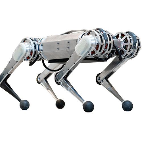
Our SLIP analysis was simplified considerably by the assumption that the leg is massless, and can be moved instantaneously during the flight phase into the desired touchdown position. This might sound to you like an offensive oversimplification, but in fact the strong trend in legged robots these days has been to build physical devices which make this sort of abstraction (approximately) valid. For quadrupeds especially, it's hard to fall over when you can move your foot instantaneously into the direction where your body is falling.
/cdn.vox-cdn.com/uploads/chorus_asset/file/16125611/bd_spotmini.jpg)
Assuming a massless leg also gives us a nice conceptual advantage -- it becomes natural to think about control design as making a control decision once per step. This fits nicely with our Poincaré analysis -- we can think of the apex-to-apex map of the SLIP model as being parameterized by the (scalar) control decision $u[n]$ which sets the touchdown angle for the $n$th hop: $$x_p[n+1] = P(x_p[n], u[n]).$$ This system can be stabilized like any other discrete-time system. For example, it would be perfectly reasonable to linearize the apex-to-apex map around the hopping fixed point, and use the (discrete-time) linear quadratic regulator to design a controller.
It turns out that for the SLIP model, there is a more interesting
approach available. If we set the cost on control effort to zero
(consistent with our massless leg assumption), then the optimal action
to pick is the one that drives the system exactly to the desired fixed
point in a single hop. This is the so-called deadbeat
controller. Not all systems can be stabilized in this way, but
Take a moment to reflect on this. In continuous time, if I were to remove the cost on control input, then the optimal actions would be unbounded, or bang-bang if there are input limits. But in discrete-time systems, this is not necessarily the case -- one can often achieve perfect convergence in a finite number of steps with bounded control input -- this corresponds to a finite-time convergence in continuous time. For this simple running model, what is particularly elegant is that this convergence can even be achieved in just one step.
In fact, the story for deadbeat control of the SLIP model gets even
better.
One would not expect to use the terms "blind", "running", "rough-terrain", and "deadbeat control" all at once to describe a control strategy. But there you have it. A very nice result! The authors went on to study whether this observation could help to explain the known phenomenon in biomechanics of "ground-speed matching" -- a human/animals' tendency to actively swing the leg around to meet the ground at the moment of touchdown.
SLIP extensions
The original SLIP model, perhaps inspired by the hopping robots
turned out to be quite effective in describing the vertical center of
mass dynamics of a wide range of animals
Hopping robots from the MIT Leg Laboratory
The 2D Hopper
A three-part control strategy: decoupling the control of hopping
height, body attitude, and forward velocity
Running on four legs as though they were one
bipeds, quadrupeds, and backflips...
Towards human-like running
A simple model that can walk and run
Juggling
Although they are not technically legged robots, there is another beautiful set
of model systems that were developed alongside some of the results that we've been
describing here, making use of the same tools and analysis. Juggling in its full
generality is, of course, a very dynamic and dexterous task that requires great
skill. But clever roboticists have found a way to distill it down to its essence

The simplest possible model is called the "line juggler", because both the robot (which here is just a simple paddle) and the single ball are constrained to move only along a line -- imagine the ball being constrained in a vertical track. We will write the robotics's configuration as $r$, the vertical distance from the horizon, and the ball's configuration as $b$, the vertical distance from the same horizon. We will assume that we have velocity control over the robot so can command $\dot{r}$ directly. When the ball is in the air, then it's dynamics are simply $\ddot{b} = -mg$. We will model the contact between the paddle and the ball as being instantantious elastic collision with coefficient of restitution, $0 \le e \le 1$.
Once again, the intermittent dynamics of the juggler are most naturally expressed
on the Poincaré map. This map can be difficult to compute in general, but
there is a clever parameterization of the action space which mitigates all of the
potential complexity. In particular,
The Line Juggler
Planar juggler
Exercises
One-Dimensional Hopper
In this exercise we implement a one-dimensional version of the controller proposed in
- A function that, given the state of the hopper, returns its total mechanical energy.
- The hopping controller class. This is a
LeafSystem that, at each sampling time, reads the state of the hopper and returns the preload of the hopper spring necessary for the system to hop at the desired height. All the necessary information for the synthesis of this controller are given in the notebook.