Model Systems with Stochasticity
My goals for this chapter are to build intuition for the beautiful and rich behavior of nonlinear dynamical system that are subjected to random (noise/disturbance) inputs. So far we have focused primarily on systems described by \[ \dot{\bx}(t) = f(\bx(t),\bu(t)) \quad \text{or} \quad \bx[n+1] = f(\bx[n],\bu[n]). \] In this chapter, I would like to broaden the scope to think about \[ \dot{\bx}(t) = f(\bx(t),\bu(t),\bw(t)) \quad \text{or} \quad \bx[n+1] = f(\bx[n],\bu[n],\bw[n]), \] where this additional input $\bw$ is the (vector) output of some random process. In other words, we can begin thinking about stochastic systems by simply understanding the dynamics of our existing ODEs subjected to an additional random input.
This form is extremely general as written. $\bw(t)$ can represent time-varying random disturbances (e.g. gusts of wind), or even constant model errors/uncertainty. One thing that we are not adding, yet, is measurement uncertainty (this will come later, when we discuss state estimation and output feedback). For this chapter we are assuming perfect measurements of the full state, and are focused instead on the way that "process noise" shapes the long-term dynamics of the system.
I will also stick primarily to discrete-time dynamics for this chapter, simply because it is easier to think about the output of a discrete-time random process, $\bw[n]$, than a $\bw(t)$. But you should know that all of the ideas work in continuous time, too. Also, most of our examples will take the form of additive noise: \[ \bx[n+1] = f(\bx[n],\bu[n]) + \bw[n], \] which is a particular useful and common specialization of our general form. And this form doesn't give up much -- the disturbance on step $k$ can pass through the nonlinear function $f$ on step $k+1$ giving rich results -- but is often much easier to work with.
When implementing stochastic systems in Drake, we aim to be rigorous about randomness, to facilitate advanced algorithms that are written against stochastic systems and to enable, e.g. random simulation roll outs but still enable deterministic replay (simulation is deterministic given the random seed).
The Master Equation
Let's start by looking at some simple examples.
A Bistable System + Noise
Let's consider (a time-reversed version of) one of my favorite
one-dimensional systems: \[ \dot{x} = x - x^3. \]
A reasonable discrete-time approximation of these dynamics, now with additive noise, is \[ x[n+1] = x[n] + h (x[n] - x[n]^3 + w[n]). \] When $w[n]=0$, this system has the same fixed points and stability properties as the continuous time system. But let's examine the system when $w[n]$ is instead the result of a zero-mean Gaussian white noise process, defined by: \begin{gather*} \forall n, E\left[ w[n] \right] = 0,\\ E\left[ w[i]w[j] \right] = \begin{cases} \sigma^2, & \text{ if } i=j,\\ 0, & \text{ otherwise.} \end{cases} \end{gather*} Here $\sigma$ is the standard deviation of the Gaussian.
When you simulate this system for small values of $\sigma$, you will see trajectories move roughly towards one of the two fixed points (for the deterministic system), but every step is modified by the noise. In fact, even if the trajectory were to arrive exactly at what was once a fixed point, it is almost surely going to move again on the very next step. In fact, if we plot many runs of the simulation from different initial conditions all on the same plot, we will see something like the figure below.

During any individual simulation, the state jumps around randomly for all time, and could even transition from the vicinity of one fixed point to the other fixed point. Another way to visualize this output is to animate a histogram of the particles over time.
You can run this demo for yourself:
Let's take a moment to appreciate the implications of what we've just observed. Every time that we've analyzed a system to date, we've asked questions like "given x[0], what is the long-term behavior of the system, $\lim_{n\rightarrow\infty} x[n]$?", but now $x[n]$ is a random variable. The trajectories of this system do not converge, and the system does not exhibit any form of stability that we've introduced so far.
All is not lost. If you watch the animation closely, you might notice the distribution of this random variable is actually very well behaved. This is the key idea for this chapter.
Let us use $p_x(x; n)$ to denote the
probability density function over the random variable $x$ at time $n$.
Note that this density function must satisfy \[ \int_{-\infty}^\infty p_x(x ;n)
dx = 1.\] It is actually possible to write the dynamics of the
probability density with the simple relation \[ p_x(x; n+1) =
\int_{-\infty}^\infty p(x|x') p_x(x'; n) dx', \] where $p(x|x')$ encodes the
stochastic dynamics as a conditional distribution of the next state (here
$x$) as a function of the current state (here $x'$). Dynamical systems that
can be encoded in this way are known as continuous-state Markov
Processes, and the governing equation above is often referred to as the
"master
equation" for the stochastic process. In fact this update is even
linear(!) ; a fact that can enable closed-form solutions to some impressive
long-term statistics, like mean time to failure or first passage
times
The Logistic Map
In fact, one does not actually need stochastic dynamics in order for
the dynamics of the distribution to be the meaningful object of study;
random initial conditions can be enough. One of the best examples comes
from perhaps the simplest and most famous example of a chaotic system: the
logistic map. This example is described beautifully in
Consider the following difference equation: $$x[n+1] = 4 x[n](1-x[n]),$$ which we will study over the (invariant) interval $x \in [0, 1]$.

It takes only a moment of tracing your finger along the plot using the "staircase method" to see what makes this system so interesting -- rollouts from a single initial condition end up bouncing all over the interval $(0,1)$, and neighboring initial conditions will end up taking arbitrarily different trajectories (this is the hallmark of a "chaotic" system).

Here's what's completely fascinating -- even though the dynamics of any one
initial condition for this system are extremely complex, if we study the dynamics
of a distribution of states through the system, they are surprisingly simple and
well-behaved. This system is one of the rare cases when we can write the master
equation in closed form

For this system (and many chaotic systems), the dynamics of a single initial condition are complicated, but the dynamics a distribution of initial conditions are beautiful and simple!
Note: when the dynamical system under study has deterministic dynamics (but a distribution of initial conditions), the linear map given by the master equation is known as the Perron-Frobenius operator, and it gives rise to the Liouville equation that we will study later in the text.
The slightly more general form of the master equation, which works for multivariate distributions with state-domain ${\cal X}$, and systems with control inputs $\bu$, is \[ p_x(\bx; n+1) = \int_{\cal X} p(\bx|\bx',\bu) p_x(\bx'; n) d\bx'. \] This is a (continuous-state) Markov Decision Process.
Continuous-time formulations are also possible -- these lead to the so-called Fokker-Planck equation.
Stationary Distributions
In the example above, the histogram is our numerical approximation of the probability density. Each of those example systems had the remarkable property that, although the individual trajectories of the system do not converge, the probability distribution actually does converge to what's known as a stationary distribution -- a fixed point of the master equation. Instead of thinking about the dynamics of the trajectories, we need to start thinking about the dynamics of the distribution.
The most important example of this analysis is for systems with linear dynamics and additive Gaussian noise; for this case we have closed-form solutions (in arbitrary dimensions). But to keep things simple, let's make sure we understand the scalar case first.
A One-dimensional Linear Gaussian System
Let's consider the one-dimensional linear system with additive noise: \[ x[n+1] = a x[n] + w[n]. \] When $w[n]=0$, the system is stable (to the origin) for $-1 < a < 1$. Let's make sure that we can understand the dynamics of the master equation for the case when $w[n]$ is Gaussian white noise with standard deviation $\sigma$.
First, recall that the probability density function of a Gaussian with mean $\mu$ is given by \[ p_w(w) = \frac{1}{\sqrt{2 \pi \sigma_w^2}} e^{-\frac{(w-\mu)^2}{2\sigma_w^2}}. \] When conditioned on $x[n]$, the distribution given by the dynamics subjected to mean-zero Gaussian white noise is simply another Gaussian, with the mean given by $ax[n]$: \[ p(x[n+1]|x[n]) = \frac{1}{\sqrt{2 \pi \sigma_w^2}} e^{-\frac{(x[n+1]-ax[n])^2}{2\sigma_w^2}}, \] yielding the master equation \[ p_{x}(x;n+1) = \frac{1}{\sqrt{2 \pi \sigma_w^2}} \int_{-\infty}^\infty e^{-\frac{(x-ax')^2}{2\sigma_w^2}} p_{x}(x';n) dx'. \]
Now here's the magic. Let's push a distribution, $p_{x}(x;n)$, which is zero-mean, with standard deviation $\sigma_n$, through the master equation: \begin{align*} p_{x}(x;n+1) =& \frac{1}{\sqrt{2 \pi \sigma_w^2}}\frac{1}{\sqrt{2 \pi \sigma_n^2}} \int_{-\infty}^\infty e^{-\frac{(x-ax')^2}{2\sigma_w^2}} e^{-\frac{(x')^2}{2\sigma_n^2}} dx',\\ =& \frac{1}{\sqrt{2 \pi (\sigma_w^2+a^2 \sigma_n^2)}} e^{-\frac{x^2}{2(\sigma_w^2 + a^2 \sigma_n^2)}}. \end{align*} The result is another mean-zero Gaussian with $\sigma_{n+1}^2 = \sigma_w^2 + a^2 \sigma_n^2$. This result generalizes to the multi-variate case, too, and might be familiar to you e.g. from the process update of the Kalman filter.
Taking it a step further, we can see that a stationary distribution for this system is given by a mean-zero Gaussian with \[ \sigma_*^2 = \frac{\sigma_w^2}{1-a^2}. \] Note that this distribution is well defined when $-1 < a < 1$. In this case, these are the same conditions we have for deterministic stability of this system.
The stationary distribution of the linear Gaussian system reveals the fundamental and general balance between two terms in the governing equations of any stochastic dynamical system: the stability of the deterministic system is bringing trajectories together (smaller $a$ means faster convergence of the deterministic system and results in a more narrow distribution), but the noise in the system is forcing trajectories apart (larger $\sigma$ means larger noise and results in a wider distribution).
Given how rich the dynamics can be for deterministic nonlinear systems, you can probably imagine that the possible long-term dynamics of the probability density are also extremely rich. If we simply flip the signs in the cubic polynomial dynamics we examined above, we'll get our next example:
The Cubic Polynomial + Noise
Now let's consider the discrete-time approximation of \[ \dot{x} = -x + x^3, \] again with additive noise: \[ x[n+1] = x[n] + h (-x[n] + x[n]^3 + w[n]). \] With $w[n]=0$, the system has only a single stable fixed point (at the origin), whose deterministic region of attraction is given by $x \in (-1,1)$. If we again simulate the system from a set of random initial conditions and plot the histogram, we will see something like the figure below.

Be sure to watch the animation. Or better yet, run the simulation for yourself by changing the sign of the derivative in the bistability example and re-running:
You can run this demo for yourself:
What is the stationary distribution for this system? In fact, there isn't one. Although we initially collect probability density around the stable fixed point, you should notice a slow leak -- on every step there is some probability of transitioning past unstable fixed points and getting driven by the unstable dynamics off towards infinity. If we run the simulation long enough, there won't be any probability density left at $x=0$.
The Stochastic Van der Pol Oscillator
One more example; this is a fun one. Let's think about one of the simplest examples that we had for a system that demonstrates limit cycle stability -- the Van der Pol oscillator -- but now we'll add Gaussian white noise, $$\ddot{q} + (q^2 - 1)\dot{q} + q = w(t),$$ Here's the question: if we start with a small set of initial conditions centered around one point on the limit cycle, then what is the long-term behavior of this distribution?

Since the long-term behavior of the deterministic system is periodic, it would be very logical to think that the state distribution for this stochastic system would fall into a stable periodic solution, too. But think about it a little more, and then watch the animation (or run the simulation yourself).
The explanation is simple: the periodic solution of the system is only orbitally stable; there is no stability along the limit cycle. So any disturbances that push the particles along the limit cycle will go unchecked. Eventually, the distribution will "mix" along the entire cycle. Perhaps surprisingly, this system that has a limit cycle stability when $w=0$ eventually reaches a stationary distribution (fixed point) in the master equation.

Finite Markov Decision Processes
In a setting where the state space and action spaces are finite, we can write the dynamics completely in terms of the transition probabilities \[p(s' | s, a) = P(s[n+1] = s' | s[n] = s, a[n] = a). \] Conveniently, we can represent the entire state probability distribution as a vector, ${\bf b}[n],$ where ${\bf b}_i[n] = p_s(s_i;n),$ and write the dynamics as a transition matrix for each action: $$T_{ij}(a) = p(s_i | s_j, a).$$ The stochastic dynamics of the master equation are then given by $${\bf b}[n+1] = {\bf T}({\bf a}[n]) {\bf b}[n].$$ Note that ${\bf T}$ is not an arbitrary matrix of real numbers but rather a (left) "stochastic matrix": we always have that $T_{ij} \in [0, 1]$ and $\sum_{i}T_{ij} = 1.$
Dynamics of a Markov chain
The dynamics of a closed-loop system (e.g. with no action inputs, or a fixed policy, $\pi$), then the MDP equations reduce back to the simpler form of a Markov chain: $${\bf b}[n+1] = {\bf T} {\bf b}[n].$$ We've already pointed out that the dynamics of the probability distribution are (action-dependent) linear; this form makes it particularly clear. To evaluate the long-term dynamics of a Markov chain, we have $${\bf b}[n] = {\bf T}^n {\bf b}[0].$$ The eigenvalues of a stochastic matrix are also bounded: $\forall i, \lambda_i \in [0, 1].$ Moreover, it can be shown that every stochastic matrix has at least one eigenvalue of $1$; any eigenvector corresponding to an eigenvalue of 1 is a stationary distribution (a fixed point of the master equation) of the Markov chain. If the Markov chain is "irreducible" and "aperiodic", then the stationary distribution is unique and the Markov chain converges to it from any initial condition.
Discretized cubic polynomial w/ noise
I used the discrete-time approximation of cubic polynomial with Gaussian noise as an example when we were first building our intuition about stochastic dynamics. Let's now make a finite-state Markov chain approximation of those dynamics, by discretizing the state space in 100 bins over the domain $x \in [-2, 2].$
Let's examine the eigenvalues of this stochastic transition matrix...
Extended Example: The Rimless Wheel on Rough Terrain
One of my favorite examples of a meaningful source of randomness on a model
underactuated system is the rimless
wheel rolling down stochastically "rough" terrain

In our original analysis of the rimless wheel, we derived the "post-collision" return map -- mapping the angular velocity from the beginning of the stance phase to the (post-collision) angular velocity at the next stance phase. But now that the relative location of the ground is changing on every step, we instead write the "apex-to-apex" return map, which maps the angular velocity from one apex (the moment that the leg is vertical) to the next, which is given by: $$\dot\theta[n+1] = \sqrt{\cos^2\alpha \left( \dot\theta^2[n] + \frac{2g}{l}\left(1-\cos(\alpha + \gamma[n])\right)\right) - \frac{2g}{l}(1 - \cos(\alpha - \gamma[n]))}.$$
More coming soon. Read the paper
Randomized smoothing of contact dynamics
It is interesting to think more generally about how stochastic dynamics interact with the contact dynamics that we have begun to study in these notes. For the stochastic rimless wheel we studied the dynamics on the apex-to-apex map, but now we'd like to consider a more typical (discrete-time, with a small, fixed, time step) model of contact dynamics.
First we have to think about a simplest reasonable model for the process
noise/dynamics. In the multibody appendix, we develop the time-stepping dynamic
models of contact as the solution to an optimization problem, which strictly
enforces contact constraints (e.g. non-penetration) at the end of every time step.
Let's use that idea again here, following the ideas developed in
A (stochastic) block near a wall
Consider the dynamics of an unactuated 1D block with a wall occupying $q \leq 0$, such that the physical dynamics is identity if the block is in a non-penetrating configuration, $q[n+1] = f(q[n])=q[n]$ if $q[n]\geq 0$. The dynamics within the penetrating regime is not well-defined physically; yet, applying the quasi-dynamic equations of motions fromThis now gives us a natural model for adding noise while respecting the non-penetration conditions. On each time step, we will apply a Gaussian perturbation (e.g. Brownian motion), $w[n]$, and apply the dynamics $q[n+1] = f(q[n] + w[n]).$ In this model, if we start the system from a known initial condition, $p_0(q) = \delta(q-q_0),$ then after one step we obtain the distribution pictured in the bottom left:
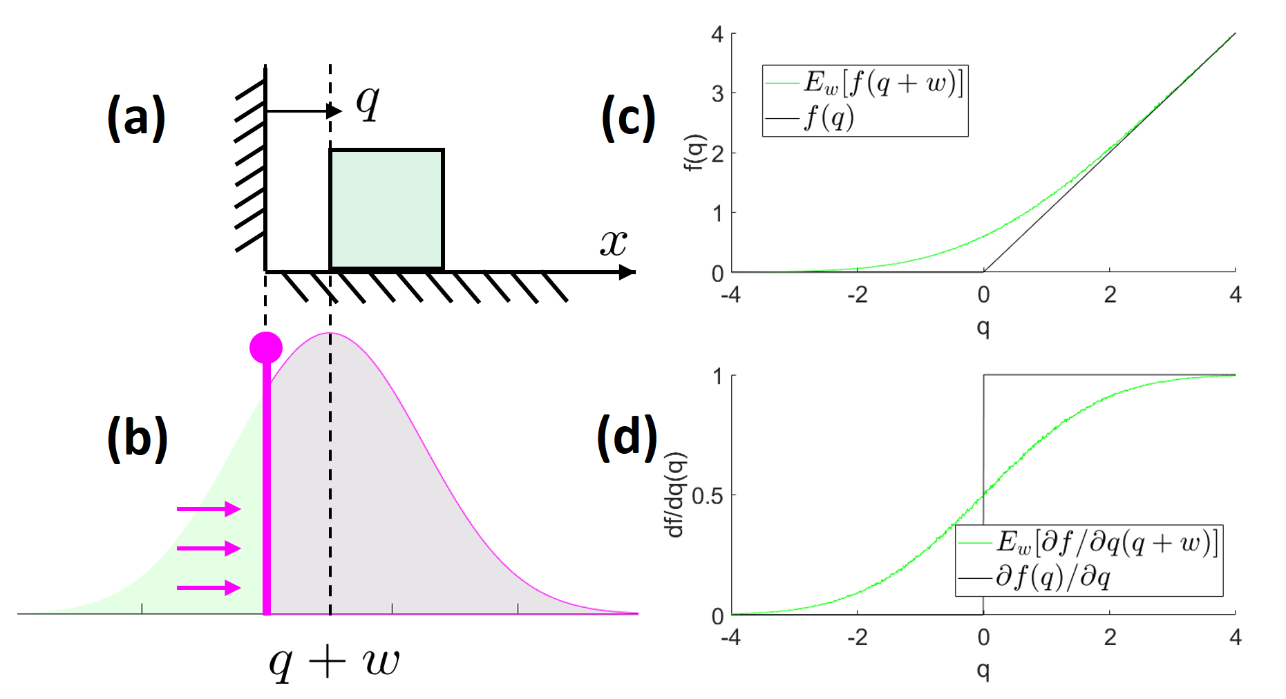
In some stochastic optimal control frameworks (and almost all reinforcement
learning algorithms), the optimization objective is specified in terms of the
expected value of the cost/reward. So it is very interesting to think about the
effect that the stochasticity has on the expected value of simulation roll-outs.
Here we see that, even after a single step, the stochasticity has the effect of
"smoothing" the hard contact dynamics, and giving a form of "contact forces at a
distance".
Interestingly, reinforcement learning (RL) algorithms often explicitly inject random perturbations (typically in the policy outputs) as a mechanism for exploring the policy parameters. When coupled with a deterministic contact simulation engine, the resulting dynamics look like the simple stochastic example illustrated above. This is one explanation for why RL has performed surprisingly well in problems involving contact dynamics.
Noise models for real robots/systems.
Sensor models. Beam model from probabilistic robotics. RGB-D dropouts.
Perception subsystem. Output of a perception system is not Gaussian noise, it's missed detections/drop-outs...
Distributions over tasks/environments. Domain randomization in RL.